In addition to including images created externally (e.g. photographs), PreTeXt supports several languages for describing diagrams and pictures with human-readable source code (i.e. plain text), rather than using a “paint” program. This section describes the various methods for incorporationg, or generating, graphis, images or diagrams.
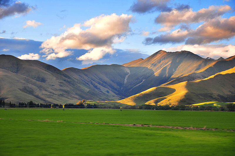
If you have existing images that are vector graphics, then PDF format works best for LaTeX output and SVG format works best for HTML. The utility pdf2svg works well for converting PDF to SVG. In this case, specify your source as a filename, but leave off the file extension, and the appropriate version will be used for the current output format.
The image below is provided from a PDF file in LaTeX output, and was converted to an SVG for use with the HTML output. It has been explicitly scaled to a width of 65% of the text width.
PreFigure is a standalone project for authoring mathematical diagrams (see prefigure.org). Its philosophy and approach are much like that of PreTeXt, and PreFigure is tightly integrated into PreTeXt. One key feature is excellent support for the creation of accessible output formats.
As of 2024-11-06 development continues for PreFigure itself, and fine-tuning of its integration within PreTeXt. But it is usable now for projects that want to use it.
You can author PreFigure diagrams, and then generate SVG, PDF, and PNG output versions with the pretext/pretext script (see the PreTeXt Guide), and expect them to render in HTML, PDF, and EPUB output formats.
Production of tactile versions is now possible, though they are not incorporated explicitly into any of the output formats. Perhaps they will become available via archive links or as a zip archive.
This next diagram employs some LaTeX macros that are defined in the usual way in <docinfo> and are employed to produce the names of some vectors in the labels. The blue line is colored blue by a global PreFigure declaration, also in <docinfo>.
The next PreFigure diagram is authored with annotations, arranged in a hierarchy of increasing refinement and detail. Each identified graphical component will read its annotation and show it on the screen below the diagram. When a reader clicks on the image, a high-level summary will be read using the author-provided annotation. The down and up arrow keys enable a reader to explore the diagram in more or less detail while the right and left arrow keys reveal features at the same level of detail. When the focus is on the graph, pressing "O" will produce a sonification of the graph.
Including annotations enables a new type of interactive diagram within a PreTeXt document offering potential benefits for all readers. In particular, annotations allow an author to call the reader’s attention to specific details in a diagram and how they are related to one another so that the diagram and surrounding text are more tightly integrated. The annotated diagram below introduces Fibonacci tilings, which are one-dimensional analogs of Penrose tilings, and offers an explanation of their aperiodicity. Of course, surrounding text would usually provide a richer context for a diagram like this.
Figure10.5.Fibonacci tilings are one-dimensional analogs of Penrose tilings. The diagram on the left introduces the process of deflation that is used to produce tilings while the diagram on the right explains why they are aperiodic.
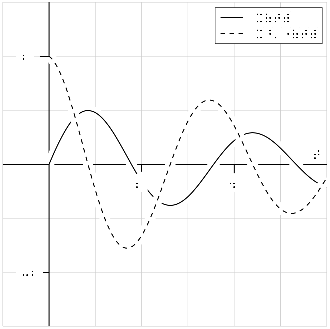
For sighted readers, here is an example of a tactile version of one of the above diagrams. It is generated automatically from the same source as the other version. Imagine this being “printed” with an embosser so that the parts of the diagram, and the braille labels, are raised up from the paper and can be explored with one’s fingertips. This image is a PNG produced specifically for this document. Typically, a tactile diagram produced by PreFigure will be a PDF ready to be sent to an appropriate embosser. Notice that PreTeXt adds a caption indicating the diagram’s location in the document along the top of the diagram.
There are several graphics engine packages that a LaTeX document can employ. Code from these packages renders diagrams automatically as part of normal processing of LaTeX files. For HTML output the pretext script produces SVG versions of the pictures. The script can also produce standalone TeX source files, PDFs, PNGs, and EPSs. The packages should be loaded in docinfo/latex-image-preamble, which is also where global package settings should be made. If any ampersands occur in your LaTeX code you should use the \amp macro pre-defined by PreTeXt. These first examples are from the TeXample.net site. Note that any LaTeX macros used in the rest of your document may be employed in the LaTeX-standalone or Asymptote diagrams (with this feature coming to Sage graphics next?).
The pgfplots package was included in docinfo/latex-image-preamble. Here, it is used. Also, here we demonstrate using \amp where you would normally use an ampersand in LaTeX. There are known issues with xelatex processing any gradient shading in tikz. To (successfully) create the gradient shading in the 3D image here, you may need to use pdflatex until LaTeX developers resolve this issue.
A plot might use a graphics language to draw the axes and grid, but the data might be from an experiment and live in an external file that you do not wish to place in your source. Place such a file in a subdirectory directly below the directory where your master source file resides. Then indicate this directory in a docinfo/directories/@data attribute of your source. But you must prefix the path with data/ as in the source below.
The TikZ image in the next figure is made up from two PNG images (the shark and the swimmer), in addition to various TikZ commands. The images reside in a source directory, numerical/attack, so the image files (shark.png, swimmer.png) are prefixed in the TikZ code with data/attack so the creation of the image will be successful. This example is courtesy of Stephen Brown.
The next image requires three passes with LaTeX to get everything in place. It is placed here to test that the code in the Pythion script correctly recognizes this requirement.
PSTricks is a LaTeX package for drawing diagrams and pictures, dating back to the days before PDF, when PostScript (PS) was king. Given its history, it does not seem to work easily with the pdflatex engine. But it will work easily with the xelatex engine. We try to keep this present sample document workable with both engines, so we have presented an example of the use of PSTricks in the xelatex-exclusive sample document where we test obscure fonts and characters. So your best bet is to look there.
The Asymptote graphics language may be placed in your source to draw graphs, diagrams or pictures. Rules for formatting code are identical to those for Sage code. For more on Asymptote see asymptote.sourceforge.net.
This is a simple physics diagram about levers, taken from the Asymptote documentation. In the HTML version of this article, the images are SVG’s and so should scale nicely when you zoom in on the page.
This diagram has two masses at either end of a lever, namely \(m\) and \(M\text{.}\) They are located at distance \(x\) and \(X\) on an axis. The resulting center-of-mass is at a point \(\bar{x}\text{.}\)
And a colorful contour plot with logarithmic scale. Again, from the Asymptote documentation. This SVG image employs two additional PNG images for the two parts where the color varies continuously.
Here is the lever diagram again, but now we have added an integral to one of the legends, using a LaTeX macro of our own, which is idential to one we used in the early part of this article. The point is, we only needed to define the macro once for the entire document, and it is available as we make Asymptote diagrams. This device can be used to maintain flexibility and consistency in your choice of notation.
Asymptote can create an HTML file that is an interactive version of a 3D shape. At this writing (2020-05-18) support via the pretext script is evolving. Plus, you will need newer versions of Asymptote and the dvisvgm utility to duplicate all of the results being displayed here in this testing document. The other distinction is that the author needs to provide the aspect ratio of the figure, and this should be placed on the <asymptote> element (not on the <image> element). Figure 10.16 is from the Asymptote Gallery.
These 3D images in HTML output are rotable with a pointing device (mouse, trackpad) with a click-and-drag. A finger should suffice on touch-sensitive devices (phones, tablets). Zooming in and out can be accomplished with a mouse wheel, or by pinching. As a contribution to the accessibility of PreTeXt HTML output, keyboard controls will also allow for exploration of these images. (Make sure the image has focus when you attempt to use these.)
And finally, an example of a 3-D graph (from the Asymptote documentation again). This WebGL image is a beautiful example of a Riemann surface. As you rotate the image, notice how the reflection of the light source varies, along with the brightness of various regions of the surface. This example is accomplished with just 10 lines of Asymptote code.
Mermaid is a Markdown-inspired tool for authoring various kinds of diagrams. Below, three of the available diagram types are demonstrated. For a full listing of diagram types, see the Mermaid Documentation. The Mermaid live editoris a great tool for testing the syntax of your mermaid diagrams.
For HTML output, if you switch back-and-forth between light-mode and dark-mode, you will need to refresh the page to see the changes in the Mermaid diagrams.
                        sequenceDiagram
                            participant Alice
                            participant Bob
                            Alice->>John: Hello John, how are you?
                            loop HealthCheck
                                John->>John: Fight against hypochondria
                            end
                            Note right of John: Rational thoughts <br/>prevail!
                            John-->>Alice: Great!
                            John->>Bob: How about you?
                            Bob-->>John: Jolly good!
Mermaid has two layout engines—the default and elk. The ELK engine often does a better job with complex diagrams. You can specify it as a default by setting the publisher variable <common/mermaid/@layout-engine> to "elk", or specify it in a single diagram by using standard Mermaid config frontmatter as shown in 10.22 below.
Any of the numerous capabilities of Sage may be used to produce any graphics object, be it the simple graph of a single-variable function or some realization of a more complicated object. All of the usual rules about formatting Sage code (esp. indentation) apply, along with one more caveat. The last line of your Sage code must return a Sage Graphics object (or 3D plot). The pretext script will isolate this last line, use it as the RHS of an assignment statement, and the Sage .save() method will be called to generate the image, which is either a Portable Document Format (PDF) file amenable to LaTeX output, or a Scalable Vector Graphics (SVG) file amenable to HTML output. For visualizations of 3D plots, Sage will only produce Portable Network Graphics (PNG) files, which can be included in HTML pages or LaTeX output. For complete documentation, see the PreTeXt Guide as this subsection is not comprehensive.
Pay careful attention to the requirement that the last line of your code be a graphics object. In particular, while show() might appear to do the right thing, it evaluates to Python’s None object and that is just what you will get. The code for Figure 10.24 illustrates creating two graphics objects and combining them into an expression on the last line that evaluates to a graphics object.
Sage code comprised of just a single line was once mishandled, leading to no ouput. From Jean-Sébastien Turcotte we have the example that revealed the problem.
in rectangular \(xyz\) coordinates, with \(t\) equal to the golden ratio. If you set plot_points=100 in the Sage code, you will get a very smooth rendering, but also a quite large HTML file. We have used plot_points=50 to reduce the file size by a factor of four. Note the need for a value of 3d for the @variant attribute, and an explicit aspect ratio with @aspect. Arrow keys, a mouse scroll wheel, plus grabbing with a left or a right mouse button, can be used to manipulate the image.
Inkscape is a great tool for creating images. It ticks all the boxes: open source, mature, cross-platform, standards-compliant. Read much more about it in The PreTeXt Guide. In HTML output the two images below are both in SVG format. The first is “pure” SVG, while the second has embedded information that makes it easier to edit in Inkscape. You could view the source for this page in the HTML version, deduce the filename of the second image, download it, and manipulate it profitably with Inkscape. Both files are quite small, but the first is half the size of the second. In PDF the two images come from files that are identical, so nothing is being tested. The PDF version is smaller still.
For images described by code, such as TikZ code in a <latex-image> element, this is a bit subtler. See the PreTeXt Guide for a complete description. We also demonstrate this with the sample book, since it is all set up with the xinclude mechanism. See the two plots of the 8-th roots of unity in the complex numbers section of the chapter on cyclic groups.
Figure10.31.A caption can be a whole paragraph with lots of technical details, and maybe a hyperlink to something external, such as pretextbook.org or PreTeXt. There could be some inline mathematics, such as \(x^2 + y^2 = c^2\text{.}\) Would a knowl open here? Recursively? Let’s see: 10.31. Display mathematics, side-by-sides, theorems, and lots of other things should be banned. Footnotes sound like a bad idea. Strange characters should be fine: §.
We strongly suggest placing images within a <figure>, as we have done above, so that you can reference them, and use the (required) <caption> to explain what they are. However there are places, such as a <preface>, where numbered items are not permitted. So you might want a solo image there. Or maybe graphics are an illustration of sorts, and a numbered figure feels like overkill. Or it is part of an <exercise> or <proof> of a <theorem>. But notice that you cannot then use this image as the target of a cross-reference, so you may need to refer to some enclosing container.
The image can be scaled by specifying the @width as a percentage, including the percent-sign (%). The height is scaled to preserve the aspect ratio. There is no facility to change the height, it is your responsibility to manage the aspect ratio independently. The @margins can be given as a pair of percentages, separated by a space. The @width defaults to 100%, while @margins defaults to the value auto, which will center the image. Missing values are computed sensibly, and there is robust error-checking. The layout control here is a subset of what is available for the more elaborate <sidebyside> element, see Section 26.
You might wish to place a single image flush-left, or flush-right. You can specify the margins attribute as a pair of percentages for different left and right margins. The following are laid out with two margins, with a 0% left margin and right margin (respectively).
All the images above are specified by filenames. We need to test how various options behave when incorporated into the (new) implementation for images, being introduced with solo images.
The table below is a summary of how graphics and images are specified, constructed and manipulated. Additional processing is indicated by reference to the Python script pretext. Images need to be placed relative to the LaTeX file that includes them during compilation, and placed relative to the HTML files which reference/include them. Author-provided image files may be placed in any subdirectory, and the @source attribute should include the complete relative path with the subdirectory. Files generated by the pretext script will be specified in the output using the relative directory images, which can be changed. There is no reason author-provided files cannot also be placed in this same directory (presuming no duplicate names). [This table is presently more readable in HTML, the PDF version will improve.]
In the early stages of a writing project, it may be best not to track provisional image files built with pretext under version control, and just regenerate them periodically (see the -r option for pretext). As a project matures, then it makes sense to put stable files under version control for collaborators and others. In every case, managing graphics files (and other aspects of production), is much more pleasurable with a script (shell, Makefile, etc.)
An <image> should either have a non-empty <description>, a non-empty <shortdescription>, or set @decorative to the value yes. Some of the following images comply, and some do not. There’s not really anything to see here visually, this is testing notifications made elsewhere.


![a standard parabola on the interval [-2,4]](generated/sageplot/sageplot-parabola.svg)


![a standard parabola on the interval [-2,4]](generated/sageplot/sageplot-parabola-solo.svg)


