Section23rd-Order Tensor Decompositions
Subsection2.1Modal Operations
To discuss the Higher Order SVD, we must first have a general understanding of two modal operations, modal unfoldings and modal products.
For a 3rd-order tensor, \(\mathcal{A} \in \mathbb{R}^{n_1 \times n_2 \times n_3}\), there are 3 modal unfoldings and in general a \(d\)-order tensor has \(d\) modal unfoldings. As a simple example the modal unfoldings for \(\mathcal{A} \in \mathbb{R}^{3 \times 4 \times 2}\) are shown below, where \(\mathcal{A}_1\) and \(\mathcal{A}_2\) are the frontal slices of \(\mathcal{A}\). \[\mathcal{A}_1 = \begin{bmatrix} 1 & 2 & 3 & 4\\ 5 & 6 & 7 & 8\\ 9 & 10 & 11 & 12 \end{bmatrix} \quad \mathcal{A}_2 = \begin{bmatrix} 13 & 14 & 15 & 16\\ 17 & 18 & 19 & 20\\ 21 & 22 & 23 & 24 \end{bmatrix} \] \[\mathcal{A}_{(1)} = \begin{bmatrix} 1 & 2 & 3 & 4 & 13 & 14 & 15 & 16\\ 5 & 6 & 7 & 8 & 17 & 18 & 19 & 20\\ 9 & 10 & 11 & 12 & 21 & 22 & 23 & 24 \end{bmatrix}\] \[\mathcal{A}_{(2)} = \begin{bmatrix} 1 & 5 & 9 & 13 & 17 & 21\\ 2 & 6 & 10 & 14 & 18 & 22\\ 3 & 7 & 11 & 15 & 19 & 23\\ 4 & 8 & 12 & 16 & 20 & 24 & \end{bmatrix}\] \[\mathcal{A}_{(3)} = \begin{bmatrix} 1 & 2 & 3 & 4 & 5 & 6 & 7 & 8 & 9 & 10 & 11 & 12 \\ 13 & 14 & 15 & 16 & 17 & 18 & 19 & 20 & 21 & 22 & 23 & 24 \end{bmatrix}\]
Using the definition of modal unfolding we can now define a modal product between a matrix and a tensor.
Definition2.2Modal Product
The modal product, denoted \(\times_{k}\), of a 3rd-order tensor \(\mathcal{A} \in \mathbb{R}^{n_1 \times n_2 \times n_3}\) and a matrix \(\textbf{U} \in \mathbb{R}^{J \times n_k}\), where \(J\) is any integer, is the product of modal unfolding \(\mathcal{A}_{(k)}\) with \(\textbf{U}\). Such that \[\textbf{B}=\textbf{U} \mathcal{A}_{(k)} = \mathcal{A} \times_{k} \textbf{U}\]These two operations will be used to generalize the standard SVD definition.
Subsection2.2Higher Order SVD (HOSVD)
Informally the Higher Order SVD is simply defined as an SVD for each of the tensors modal unfoldings.
Definition2.3Higher Order SVD
Suppose \(\mathcal{A}\) is a 3rd-order tensor and \(\mathcal{A} \in \mathbb{R}^{n_1 \times n_2 \times n_3}\). Then there exists a Higher Order SVD such that \[\textbf{U}^{T}_{k}\mathcal{A}_{(k)}=\Sigma_{k} \textbf{V}^{T}_{k} \quad (1\leq k \leq d)\] where \(\textbf{U}_{k}\) and \(\textbf{V}_{k}\) are unitary matrices and the matrix \(\Sigma_{k}\) contains the singular values of \(\mathcal{A}_{(k)}\) on the diagonal, \([\Sigma_{k}]_{ij}\) where \(i=j\), and is zero elsewhere.Using this definition, computing an HOSVD for a tensor of order-\(N\) is only as computationally difficult as performing \(N\) matrix SVD's. In practice the SVD of a matrix is useful in compressing a matrix to a representation that is arbitrarily close to the original. Generalizing this to the higher order tensor case can be accomplished by using the unitary matrices \(U_k\) from the HOSVD to find a tensor \(\mathcal{S}\) as follows: (the \(\rightarrow\) is used to denote undoing a modal unfolding) \begin{align*} \textbf{U}^{T}_{1} \mathcal{A}_{(1)} &= \hat{\mathcal{A}}_{(1)} \rightarrow \hat{\mathcal{A}}\\ \textbf{U}^{T}_{2} \hat{\mathcal{A}}_{(2)} & = \hat{\hat{\mathcal{A}}}_{(2)} \rightarrow \hat{\hat{\mathcal{A}}}\\ \textbf{U}^{T}_{3} \hat{\hat{\mathcal{A}}}_{(3)} &= \mathcal{S}_{(3)} \rightarrow \mathcal{S} \end{align*} This can be denoted by sequential modal products much more concisely. \begin{align*} \mathcal{S} &=\mathcal{A}\times_1 U^{T}_{1} \times_2 U^{T}_{2} \times_3 U^{T}_{3}\\ \mathcal{A} &=\mathcal{S}\times_1 U_{1} \times_2 U_{2} \times_3 U_{3} \end{align*}
This \(\mathcal{S}\) tensor is referred to as the core tensor. While this tensor is not diagonal the entries tend to decrease as distance from the diagonal increases where the diagonal is the entries from the upper left hand corner of the cube to the lower right hand corner. This property is useful when compressing the original \(\mathcal{A}\) because the dimension of \(U\) can be reduced by dropping the smaller terms, and a close approximation will still be generated, much like the compression of a matrix using SVD. The biggest example of this is the compression of color photos where each frontal slice corresponds to intensities of red, green, or blue instead of the matrix example where entries correspond to intensities on the gray-scale. This approach could also be used to first compress a tensor, then perform a CP decomposition on the compressed tensor to save computational resources.
Subsection2.3Rank of Higher Order Tensors
The notion of rank with respect to higher order tensors is not as simple as the rank of a matrix.
Definition2.4Rank of a Tensor
The rank of a tensor\(\mathcal{A}\) is the smallest number of rank 1 tensors that sum to \(\mathcal{A}\).This definition of rank comes up naturally within many of the common tensor decompositions. For example, in the CANDECOMP/PARAFAC (CP) decomposition the rank specifies the minimum number of vector outer products required to reproduce the tensor exactly. And, with a somewhat circular claim, an exact CP decomposition with minimal vector outer products can be used to determine the rank of a tensor, this is also referred to as a rank decomposition. While the definition for matrix rank is an analog to tensor rank, the properties are quite different. For example, there is no general algorithm to determine the rank of a given higher order tensor. There is only a loose upper bound on the rank of a 3rd-order tensor, \(\mathcal{A}\in\mathbb{R}^{I\times J\times K}\), described by \(rank(\mathcal{A})\leq \mbox{min}\{IJ,IK,JK\}\), but the rank is often lower than this for randomly generated tensors [4.7].
Subsection2.4CANDECOMP/PARAFAC Decomposition
Unfortunately there is no single algorithm to perform a CP decomposition on any tensor. This is partially due to the fact that the rank of a higher order tensor is not known precisely until a CP decomposition has been performed and is known to be the most concise decomposition.
Definition2.5CP Decomposition
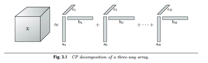
A CP decomposition of a 3rd-order tensor, \(\mathcal{A}\), is defined as a sum of vector outer products, denoted \(\circ\), that equal or approximately equal \(\mathcal{A}\). For \(R = rank(\mathcal{A})\)\[\mathcal{A} = \sum_{r=1}^{R}a_r \circ b_r \circ c_r\] and for \(R \lt rank(\mathcal{A})\)\[\mathcal{A} \approx \sum_{r=1}^{R}a_r \circ b_r \circ c_r\]The CP decomposition is nicely visualized by Kolda and Bader (2009) in Figure 3.1.
The vectors of a CP composition, \(a_r\), \(b_r\), and \(c_r\) for \(1 \leq r \leq R\), are often compiled into the columns of the matrices \(\textbf{A}\), \(\textbf{B}\), and \(\textbf{C}\) respectively, and the CP decomposition is written more concisely, \[\mathcal{A}=[[\textbf{A},\textbf{B},\textbf{C}]]\]. This type of matrix multiplication is often denoted by the \(\odot\) symbol. For instance, \[\textbf{A} \odot \textbf{B} = [a_1|a_2|\dots|a_n] \odot [b_1|b_2|\dots|b_n] = [a_1 \circ b_1|a_2 \circ b_2|\dots|a_n \circ b_n]\] The example below, from Bader and Kolda (2009), demonstrates why the rank of a matrix is difficult to determine precisely. In this example a CP decomposition over the real and complex fields is performed for \(\mathcal{A} \in \mathbb{R}^{2 \times 2 \times 2}\) where \(\mathcal{A}_1\) and \(\mathcal{A}_2\) are the frontal slices of \(\mathcal{A}\) [4.3].
\begin{align*} \mathcal{A}_1 &= \begin{bmatrix} 1 & 0\\0 & 1 \end{bmatrix} &\mathcal{A}_2 &= \begin{bmatrix} 0 & 1\\-1 & 0 \end{bmatrix} \end{align*}
The rank decomposition over \(\mathbb{R}\) is \(\mathcal{A}= [[\textbf{A},\textbf{B},\textbf{C}]]\), where \begin{align*} \textbf{A}&=\begin{bmatrix} 1 & 0 & 1\\0 & 1 & -1\end{bmatrix} & \textbf{B}&=\begin{bmatrix} 1 & 0 & 1\\0 & 1 & 1\end{bmatrix} & \textbf{C} &= \begin{bmatrix} 1 & 1 & 0\\-1 & 1 & 1\end{bmatrix} \end{align*} but over \(\mathbb{C}\) \begin{align*} \textbf{A}&=\frac{1}{\sqrt{2}}\begin{bmatrix} 1 & 1\\-i & i \end{bmatrix} & \textbf{B}&=\frac{1}{\sqrt{2}}\begin{bmatrix} 1 & 1\\i & -i \end{bmatrix} & \textbf{C}&=\begin{bmatrix} 1 & 1\\i & -i \end{bmatrix}. \end{align*}
This leads to a very surprising property, the rank of a tensor can be different over \(\mathbb{R}\) and \(\mathbb{C}\). For this reason I have restricted the definitions to \(\mathbb{R}\) to remove this ambiguity.
Performing a CP decomposition on a 3rd order tensor \(\mathcal{A}\) is a matter of performing a Alternating Least Squares (ALS) routine to minimize \(||\mathcal{A}_{(1)} - \textbf{A}(\textbf{C}\odot \textbf{B})^T||\). To perform an ALS routine on this system, the system is divided into 3 standard least squares problems where 2 of the 3 matrices are held constant and the third is solved for. The main problem in implementing an ALS routine such as this, is choosing initial values for the two matrices that are held constant to initialize the first least squares problem. This method may take many iterations to converge, the point of convergence is heavily reliant on the initial guess, and the computed solution is not always accurate. Faber, Bro, and Hopke (2003) investigated six methods as an alternative to the ALS method and none of them came out more effective than ALS in terms of accuracy of solution, but some did converge faster [4.6]. In addition, derivative methods have been developed that are superior to the ALS method in terms of convergence and solution accuracy but are much more computationally expensive [4.3]. For quantum mechanical problems involving a few \(3 \times 3 \times 3\) tensors accuracy is paramount to computational expense. One such algorithm is the PMF3 algorithm described in Paatero (1997) which computes changes to all three matrices simultaneously. This allows for faster convergence than the ALS method and optional specificity for non-negative solutions reduces divergence in systems that are known to have positive solutions [4.5].