Derivatives and Integrals: An Annotated Discourse

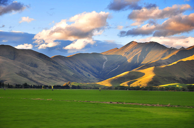
All by itsef, with no layout specified, so showing the default size and placement. Vivamus in congue massa. Morbi condimentum ac magna at accumsan. Vestibulum ac augue eu lorem semper gravida.

Width set at 40%, so equal margins and thus centered. Aenean faucibus augue tellus, et sollicitudin tortor finibus non. Maecenas semper dolor quis diam placerat, iaculis sollicitudin augue finibus. Vestibulum facilisis ligula lectus, ac tristique nisl aliquet non.

Asymmetric margins of 20% and 40% given, implying 40% width, equal to previous instance. Vivamus suscipit diam eget mi cursus viverra.

As a plain component of a <sidebyside>. Widths here are 20% and 30%, margins and gaps are automatic, default alignment on top edges. Nulla pharetra imperdiet elit, in sodales nibh blandit ultricies. Maecenas efficitur ac felis ut pharetra.

Inside a <figure> with no adjustments, so default behavior. Note how a <figure> occupies the entire width of the page, so then does the caption.

Inside a <figure> with asymmetric (large) margins of 30% and 60%. Quisque finibus augue sit amet facilisis fringilla. Aenean faucibus augue tellus, et sollicitudin tortor finibus non.

Inside figures inside a <sidebyside>. Same widths as previous <sidebyside> but alignment on bottoms of the panels, to partially align captions. Note how the captions are constrained in width by the width of the panels of the side-by-side.

Identical code to previous example, but now wrapped in an overall <figure>, which has its own caption and number, leaving the interior figures to be sub-numbered. Cross-references use the full number: Figure 28.5.(b).

A rotation="n" attribute applied to a bare image will rotate the image by n°. The vertical space adjusts to accomodate the rotated image in the latex version but not in the html version.

For pdf output destined for print, i.e. when the publication file entry latex/@print="yes", a @landscape="yes" attribute applied to a <figure>, <table>, <list> or <listing> will cause the object to be rotated 90° and presented on its own page. Placement of the float is determined by LaTeX and multipage objects are not supported.

Videos can be realized in many forms, and can come from a variety of sources. See Section 18 for tests of some of that variety. Here we are testing placement within surroundings and testing the schema for location. But we do have two videos in each test, one provided as a local file and one embedded from a service.

All by itsef, with no layout specified, so showing the default size and placement. Vivamus in congue massa. Morbi condimentum ac magna at accumsan. Vestibulum ac augue eu lorem semper gravida.

Vestibulum facilisis ligula lectus, ac tristique nisl aliquet non. Quisque ornare felis arcu. Vivamus suscipit diam eget mi cursus viverra.

Width set at 40%, so equal margins and thus centered. Aenean faucibus augue tellus, et sollicitudin tortor finibus non. Maecenas semper dolor quis diam placerat, iaculis sollicitudin augue finibus. Vestibulum facilisis ligula lectus, ac tristique nisl aliquet non.

Vestibulum facilisis ligula lectus, ac tristique nisl aliquet non. Quisque ornare felis arcu. Vivamus suscipit diam eget mi cursus viverra.

Asymmetric margins of 20% and 40% given, implying 40% width, equal to previous instance. Vivamus suscipit diam eget mi cursus viverra.

Vestibulum facilisis ligula lectus, ac tristique nisl aliquet non. Quisque ornare felis arcu. Vivamus suscipit diam eget mi cursus viverra.

As a plain component of a <sidebyside>. Widths here are 20% and 30%, margins and gaps are automatic, default alignment on top edges. Nulla pharetra imperdiet elit, in sodales nibh blandit ultricies. Maecenas efficitur ac felis ut pharetra.

Inside a <figure> with no adjustments, so default behavior. Note how a <figure> occupies the entire width of the page, so then does the caption.

Vestibulum facilisis ligula lectus, ac tristique nisl aliquet non. Quisque ornare felis arcu. Vivamus suscipit diam eget mi cursus viverra.

Inside a <figure> with asymmetric (large) margins of 30% and 60%. Quisque finibus augue sit amet facilisis fringilla. Aenean faucibus augue tellus, et sollicitudin tortor finibus non.

Vestibulum facilisis ligula lectus, ac tristique nisl aliquet non. Quisque ornare felis arcu. Vivamus suscipit diam eget mi cursus viverra.

Inside figures inside a <sidebyside>. Same widths as previous <sidebyside> but alignment on bottoms of the panels, to partially align captions. Note how the captions are constrained in width by the width of the panels of the side-by-side.

Identical code to previous example, but now wrapped in an overall <figure>, which has its own caption and number, leaving the interior figures to be sub-numbered. Cross-references use the full number: Figure 28.16.(b).

Programs can be realized in many forms, and can come from a variety of sources. See Section 18 for tests of some of that variety. Here we are testing placement within surroundings and testing the schema for location. But we do have two videos in each test, one provided as a local file and one embedded from a service.

All by itsef, with no layout specified, so showing the default size and placement. Vivamus in congue massa. Morbi condimentum ac magna at accumsan. Vestibulum ac augue eu lorem semper gravida.

n_loops <- 10
x.means <- numeric(n_loops)  # create a vector of zeros for results
for (i in 1:n_loops){
x <- as.integer(runif(100, 1, 7))  # 1 to 6, uniformly
x.means[i] <- mean(x)
}
x.means

Now a program with shorter lines, with no layout control.

/* Hello World program */
#include<stdio.h>
main()
{
printf("Hello, World!");
}

And a <console> element, also with no layout control.

pi@raspberrypi ~/progs/chap02 $ gcc -o intAndFloat intAndFloat.c
pi@raspberrypi ~/progs/chap02 $ ./intAndFloat
The integer is 19088743 and the float is 19088.742188
pi@raspberrypi ~/progs/chap02 $ 

Now similar examples, but with layout control: margins and width.

A <program> with a @width attribute, so centered and with equal margins. Note how the lines word wrap due to the smaller width.

n_loops <- 10
x.means <- numeric(n_loops)  # create a vector of zeros for results
for (i in 1:n_loops){
x <- as.integer(runif(100, 1, 7))  # 1 to 6, uniformly
x.means[i] <- mean(x)
}
x.means

A <program> with short lines, so significant, and asymmetric margins, which experimentally do not induce any word-wrapping.

/* Hello World program */
#include<stdio.h>
main()
{
printf("Hello, World!");
}

A longer <console>, with margins so significant the appearance is ill-advised.

pi@raspberrypi ~/progs/chap02 $ gcc -Wall -o intAndFloat intAndFloat.c
pi@raspberrypi ~/progs/chap02 $ ./intAndFloat
The integer is 19088743 and the float is 19088.742188
pi@raspberrypi ~/progs/chap02 $ 

Two <listing>, with <caption>, and no layout control.

/* Hello World program */
#include<stdio.h>
main()
{
printf("Hello, World!");
}

pi@raspberrypi ~/progs/chap02 $ gcc -Wall -o intAndFloat intAndFloat.c
pi@raspberrypi ~/progs/chap02 $ ./intAndFloat
The integer is 19088743 and the float is 19088.742188
pi@raspberrypi ~/progs/chap02 $ 

Same two <listing>, but now with layout control on the <program> and <console>.

/* Hello World program */
#include<stdio.h>
main()
{
printf("Hello, World!");
}

pi@raspberrypi ~/progs/chap02 $ gcc -Wall -o intAndFloat intAndFloat.c
pi@raspberrypi ~/progs/chap02 $ ./intAndFloat
The integer is 19088743 and the float is 19088.742188
pi@raspberrypi ~/progs/chap02 $ 

This <sidebyside> gives each panel a 30% width. The remaining 10% is apportioned for margins and separation.

/* Hello World program */
#include<stdio.h>
main()
{
printf("Hello, World!");
}

pi@raspberrypi ~/progs/chap02 $ gcc -Wall -o intAndFloat intAndFloat.c
pi@raspberrypi ~/progs/chap02 $ ./intAndFloat
The integer is 19088743 and the float is 19088.742188
pi@raspberrypi ~/progs/chap02 $ 

n_loops <- 10
x.means <- numeric(n_loops)  # create a vector of zeros for results
for (i in 1:n_loops){
x <- as.integer(runif(100, 1, 7))  # 1 to 6, uniformly
x.means[i] <- mean(x)
}
x.means

This is the same three-panel <sidebyside>, but now inside of a <figure>, earning a number and a <caption>.

/* Hello World program */
#include<stdio.h>
main()
{
printf("Hello, World!");
}

pi@raspberrypi ~/progs/chap02 $ gcc -Wall -o intAndFloat intAndFloat.c
pi@raspberrypi ~/progs/chap02 $ ./intAndFloat
The integer is 19088743 and the float is 19088.742188
pi@raspberrypi ~/progs/chap02 $ 

n_loops <- 10
x.means <- numeric(n_loops)  # create a vector of zeros for results
for (i in 1:n_loops){
x <- as.integer(runif(100, 1, 7))  # 1 to 6, uniformly
x.means[i] <- mean(x)
}
x.means

Finally, a smaller <program> and a smaller <console>, each inside a <listing>, as the two panels of a <sidebyside> with no margins, and slightly different widths (to control word-wrapping). The panels have been aligned vertically so their captions align.

/* Hello World program */
#include<stdio.h>
main()
{
printf("Hello, World!");
}

$ gcc -Wall -o intAndFloat intAndFloat.c
$ ./intAndFloat
The integer is 19088743 and the float is 19088.742188
$ 

And again, the two-panel <sidebyside> of <listing>, but now inside a <figure> that has a number and a caption. And then the <listing> are sub-numbered as (a) and (b).

/* Hello World program */
#include<stdio.h>
main()
{
printf("Hello, World!");
}

$ gcc -Wall -o intAndFloat intAndFloat.c
$ ./intAndFloat
The integer is 19088743 and the float is 19088.742188
$ 

A <tabular> realized by LaTeX for PDF/print will normally be as wide as necessary to hold the content, without word-wrapping the content of any cell that is not explicitly authored that way. This is the most rigid of the content types we call “planar.” So for PreTeXt output as LaTeX, when you explicitly constrain the width to be less than the “natural width” (including use as a panel of a <sidebyside>, or even setting margins) the table will be scaled down in width, which can result in an apparent font size very much smaller than that of the surrounding text. Note that we do not ever scale a tabular up to be wider with a larger font size. Note also that if there is no attempt to control the space for the table (no layout control, not in a <sidebyside>) then no scaling is attempted at all and the table may be wider than the text and protrude into the right margin. For more, see the three examples at: Table 28.29 , Table 28.30, Table 28.31. Generally, much of the commentary and testing here is about LaTeX/PDF/print. While for HTML output the cells will usually automatically word-wrap to fit in the available space, without adjusting the font size. Some might like this behavior and some might not.

Data in a table form can be placed in amongst a series of paragraphs. With no layout control, it will occupy its “natural width” and be centered.

The same effect can be had by specifying that the @width attribute have the value auto, but do not specify any @margins. We test multiple footnotes in a <tabular>, not included in a <table>.

In amongst a run of paragraphs (or similar) a <tabular> can be placed with layout control. For LaTeX output, this will scale the table to fit within the explicit, or implicit, width. This can result in obvious differences in the apparent font size. We first have a @width that is experimentally similar to the natural width, with asymetric margins. Then a narrow width, and a wide width, as an illustration.

Narrow. 45% width. 20% margin left, 35% margin right.

Wide. 97% width. 1% margin left, 2% right.

Naturally, a <tabular> can be placed inside a <table>, earning a number and a title.

A little narrower, but still centered by default.

Very narrow, asymmetric margins.

Wider than necessary, asymmetric margins.

The next table is purposely much too wide. In Table 28.29 we make no attempt to control the width, and so it will extend into the margins. In Table 28.30 we have simple added the attribute width="auto". This attempt to use layout control will cause an automatic reduction in width and a smaller apparent font size. Adjusting margins providing an explicit percentage width, or placing the tabular as a panel of <sidebyside> will have the same effect. In Table 28.31 we have set the width explicity to 100% and so it should be identical to the automatic width case just prior.

Now into <sidebyside> in various ways and with various sizes. First, two <tabular> as panels with widths at 60% and 30%. Note that in LaTeX/PDF/print the tabular of functional values does not need the full 30% width, so it is at its natural size and centered within its panel.

Let’s do that again, but with widths experimentally set to make font sizes match (approximately).

Same tabular, which fills roughly 80% by itself, packed into a single <sidebyside> with just a 2% gap, and no side margins.

Natural widths, but now as a pair of tables.

Finally, as two individual <table>, grouped and laid out via a <sidebyside>, and collected as a <figure>. Which causes sub-numbering of the two enclosed <table>.