<section xml:id="graphics" label="section-graphics">
<title>Graphics</title>
<introduction>
<p>
In addition to including images created externally (e.g.
photographs), <pretext/> supports several languages for describing diagrams and pictures with human-readable source code (<ie/> plain text), rather than using a <q>paint</q> program.
This section describes the various methods for incorporationg, or generating, graphis, images or diagrams.
</p>
</introduction>
<subsection>
<title>Images from External Sources</title>
<p>
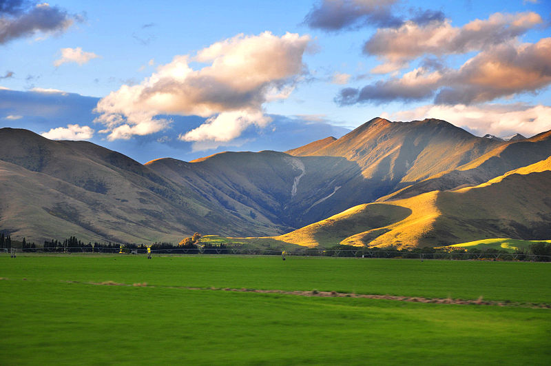
If you have raster images (photographs, etc.) then they are specified with complete filenames, as above in <xref ref="figure-function-derivative"/> or just below.
</p>
<figure>
<caption>New Zealand Landscape, <url href="https://commons.wikimedia.org/wiki/File:NZ_Landscape_from_the_van.jpg" visual="commons.wikimedia.org/wiki/File:NZ_Landscape_from_the_van.jpg"><c>commons.wikimedia.org</c></url>, CC-BY-SA-2.0</caption>
<image source="images/nz-landscape.jpg" width="80%"/>
</figure>
<p>
If you have existing images that are vector graphics, then PDF format works best for <latex/> output and SVG format works best for HTML.
The utility <c>pdf2svg</c> works well for converting PDF to SVG.
In this case, specify your source as a filename, but leave off the file extension, and the appropriate version will be used for the current output format.
</p>
<p>
The image below is provided from a PDF file in <latex/> output, and was converted to an SVG for use with the HTML output.
It has been explicitly scaled to a width of 65% of the text width.
It has a <tag>description</tag>, but no <tag>shortdescription</tag>, so is testing that scenario.
</p>
<figure xml:id="figure-complete-graph">
<caption>Complete graph on <m>16</m> vertices, from <c>www.texample.net</c></caption>
<image source="images/complete-graph" width="65%">
<description>
<p>
A circular arrangment of <m>16</m> dots (<term>vertices</term>) with <m>120</m> straight lines (<term>edges</term>), joining every pair of dots.
</p>
</description>
</image>
</figure>
<remark>
<title>Footnote Buried</title>
<p>
Nested <c>tcolorbox</c> (in <latex/> conversion) need special care when footnotes are interior.
</p>
<sidebyside margins="20% 30%">
<p>
A paragraph interior to a <c>sidebyside</c> with a footnote<fn>Interior footnote.</fn> buried inside the paragraph.
</p>
<p>
A second paragraph, just to avoid a one-panel warning.
</p>
</sidebyside>
<p>
The final paragraph of this remark, randomly placed, to test footnotes in <latex/> conversions.
</p>
</remark>
</subsection>
<subsection xml:id="prefigure-diagrams" label="prefigure-diagrams">
<title><prefigure/></title>
<idx><prefigure/>
image</idx>
<idx><h>image</h><h><prefigure/>
image</h></idx>
<p>
<prefigure/> is a standalone project for authoring mathematical diagrams (see <url href="https://prefigure.org/" visual="prefigure.org"/>). Its philosophy and approach are much like that of <pretext/>, and <prefigure/> is tightly integrated into <pretext/>. One key feature is excellent support for the creation of accessible output formats.
</p>
<p>
As of 2024-11-06 development continues for <prefigure/> itself, and fine-tuning of its integration within <pretext/>.
But it is usable now for projects that want to use it.
<ul>
<li>
You can author <prefigure/> diagrams, and then generate <init>SVG</init>, <init>PDF</init>, and <init>PNG</init> output versions with the <c>pretext/pretext</c> script (see the <pretext/> Guide), and expect them to render in <init>HTML</init>, <init>PDF</init>, and <init>EPUB</init> output formats.
</li>
<li>
Look for automatic generation to come to the <pretext/>-CLI sometime very soon.
</li>
<li>
<prefigure/> has excellent support for annotations within an <init>SVG</init> diagram, supporting their use by screenreaders, for example. See an example below.
</li>
<li>
Production of tactile versions is now possible, though they are not incorporated explicitly into any of the output formats.
Perhaps they will become available via archive links or as a zip archive.
</li>
</ul>
</p>
<p>
This is a basic <prefigure/> diagram, in the sense that it does not use all the features of <prefigure/> or <pretext/>.
</p>
<figure>
<caption>Solution to a differential equation</caption>
<image width="60%">
<prefigure label="prefigure-diffeq" xmlns="https://prefigure.org">
<diagram dimensions="(300,300)" margins="5">
<definition>
f(t,y) = (y[1], -pi*y[0]-0.3*y[1])
</definition>
<coordinates bbox="[-1,-3,6,3]">
<grid-axes xlabel="t"/>
<de-solve function="f" t0="0" t1="bbox[2]" y0="(0,2)" name="oscillator" N="200"/>
<plot-de-solution at="x" solution="oscillator" axes="(t,y0)"/>
<plot-de-solution at="xprime" solution="oscillator" axes="(t,y1)" stroke="red" tactile-dash="9 9"/>
<legend at="legend" anchor="(bbox[2], bbox[3])" alignment="sw" scale="0.9" opacity="0.5">
<item ref="x"><m>x(t)</m></item>
<item ref="xprime"><m>x'(t)</m></item>
</legend>
</coordinates>
</diagram>
</prefigure>
</image>
</figure>
<p>
This next diagram employs some <latex/> macros that are defined in the usual way in <tag>docinfo</tag> and are employed to produce the names of some vectors in the labels.
The blue line is colored blue by a global <prefigure/> declaration, also in <tag>docinfo</tag>.
</p>
<image width="60%">
<prefigure label="prefigure-projection" xmlns="https://prefigure.org">
<diagram dimensions="(300,300)" margins="5">
<definition>
v=(2,1)
</definition>
<definition>
b=(2,4)
</definition>
<definition>
bhat=dot(v,b)/dot(v,v) * v
</definition>
<definition>
bperp = b - bhat
</definition>
<coordinates bbox="[-1,-1,5,5]">
<grid-axes/>
<line endpoints="((0,0),v)" infinite="yes"/>
<label anchor="(4.4,2.5)">
<m>L</m>
</label>
<vector v="bperp" tail="bhat" stroke="gray"/>
<label anchor="midpoint(b,bhat)" alignment="ne">
<m>\bvec^\perp</m>
</label>
<vector v="b"/>
<label anchor="b" alignment="nw">
<m>\bvec</m>
</label>
<vector v="bhat" stroke="red"/>
<label anchor="bhat" alignment="se">
<m>\widehat{\bvec}</m>
</label>
<vector v="v"/>
<label anchor="v" alignment="se">
<m>\vvec</m>
</label>
</coordinates>
</diagram>
</prefigure>
</image>
<p>
The next <prefigure/> diagram is authored with annotations, arranged in a hierarchy of increasing refinement and detail.
Each identified graphical component will read its annotation and show it on the screen below the diagram.
When a reader clicks on the image, a high-level summary will be read using the author-provided annotation.
The down and up arrow keys enable a reader to explore the diagram in more or less detail while the right and left arrow keys reveal features at the same level of detail.
When the focus is on the graph, pressing "O" will produce a sonification of the graph.
</p>
<image width="60%">
<prefigure label="prefigure-tangent" xmlns="https://prefigure.org">
<diagram dimensions="(300,300)" margins="5">
<definition>
a=1
</definition>
<definition>
f(x) = exp(x/3)*cos(x)
</definition>
<coordinates bbox="[-4,-4,4,4]">
<grid-axes xlabel="x" ylabel="y"/>
<graph at="graph" function="f"/>
<tangent-line at="tangent" function="f" point="a"/>
<point at="point" p="(a, f(a))">
<m>(a,f(a))</m>
</point>
</coordinates>
<annotations text="The graph of a function and its tangent line at the point a equals 1">
<annotation ref="graph-tangent" text="The graph and its tangent line">
<annotation ref="graph" text="The graph of the function f" sonify="yes"/>
<annotation ref="point" text="The point a comma f of a"/>
<annotation ref="tangent" text="The tangent line to the graph of f at the point"/>
</annotation>
</annotations>
</diagram>
</prefigure>
</image>
<p>
Including annotations enables a new type of interactive diagram within a <pretext/> document offering potential benefits for all readers.
In particular, annotations allow an author to call the reader's attention to specific details in a diagram and how they are related to one another so that the diagram and surrounding text are more tightly integrated.
The annotated diagram below introduces Fibonacci tilings, which are one-dimensional analogs of Penrose tilings, and offers an explanation of their aperiodicity.
Of course, surrounding text would usually provide a richer context for a diagram like this.
</p>
<figure xml:id="figure-fibonnaci-tiling-annotated">
<caption>Fibonacci tilings are one-dimensional analogs of Penrose tilings. The diagram on the left introduces the process of deflation that is used to produce tilings while the diagram on the right explains why they are aperiodic.</caption>
<sidebyside widths="30% 50%" valign="bottom" margins="0% 15%">
<image>
<prefigure label="prefigure-fibonacci-a" xmlns="https://prefigure.org">
<diagram dimensions="(200, 200)">
<definition>
phi=(sqrt(5)+1)/2
</definition>
<definition>
height=0.25
</definition>
<definition>
top=1
</definition>
<definition>
bottom=0
</definition>
<definition>
left=0
</definition>
<definition>
right=2
</definition>
<definition>
colors={0:'blue', 1:'red'}
</definition>
<definition>
widths={0:phi, 1:1}
</definition>
<coordinates bbox="(-0.5,-1,3.5,2)">
<transform>
<!-- Define the upper row of tiles-->
<translate by="(0,top)"/>
<!-- We put tiles and their labels into a group for annotating-->
<group at="top-L">
<rectangle lower-left="(0,0)" dimensions="(widths[0], height)" fill="${colors[0]}" stroke="black"/>
<label anchor="(widths[0]/2,height)" alignment="n">
<m>L</m>
</label>
</group>
<translate by="(right,0)"/>
<group at="top-S">
<rectangle lower-left="(0,0)" dimensions="(widths[1],height)" fill="${colors[1]}" stroke="black"/>
<label anchor="(widths[1]/2, height)" alignment="n">
<m>S</m>
</label>
</group>
</transform>
<transform>
<translate by="(0,bottom)"/>
<transform>
<scale by="(1/phi, 1)"/>
<group at="bottom-L">
<group at="bottom-LL">
<rectangle lower-left="(0,0)" dimensions="(widths[0], height)" fill="${colors[0]}" stroke="black"/>
<label anchor="(widths[0]/2,0)" alignment="south">
<m>L</m>
</label>
</group>
<translate by="(widths[0],0)"/>
<group at="bottom-LS">
<rectangle lower-left="(0,0)" dimensions="(widths[1], height)" fill="${colors[1]}" stroke="black"/>
<label anchor="(widths[1]/2,0)" alignment="south">
<m>S</m>
</label>
</group>
</group>
</transform>
<translate by="(right, 0)"/>
<scale by="(1/phi,1)"/>
<group at="bottom-S">
<group at="bottom-SL">
<rectangle lower-left="(0,0)" dimensions="(widths[0], height)" fill="${colors[0]}" stroke="black"/>
<label anchor="(widths[0]/2,0)" alignment="south">
<m>L</m>
</label>
</group>
</group>
</transform>
<line at="left-arrow" endpoints="((left+phi/2, top), (left+phi/2, bottom+height))" endpoint-offsets="(3,-5)" arrows="1" stroke="black"/>
<line at="right-arrow" endpoints="((right+1/2, top), (right+1/2, bottom+height))" endpoint-offsets="(3,-5)" arrows="1" stroke="black"/>
</coordinates>
<annotations text="The set of Fibonacci tiles consists of two tiles denoted by L and S.">
<annotation ref="top" text="The ratio of the lengths of the tiles is the golden ratio so one tile L is long and the other S is short">
<annotation ref="top-L" text="The long tile L"/>
<annotation ref="top-S" text="The short tile S"/>
</annotation>
<annotation ref="arrows" text="A process called deflation replaces each tile by a new set of tiles">
<annotation ref="left-deflate" text="A long tile is replaced by a long and a short tile">
<annotation ref="left-arrow"/>
<annotation ref="top-L"/>
<annotation ref="bottom-L" text="The length of the new tiles is scaled by the reciprocal of the golden ratio">
<annotation ref="bottom-LL" text="The new long tile is on the left"/>
<annotation ref="bottom-LS" text="The new short tile is on the right"/>
</annotation>
</annotation>
<annotation ref="right-deflate" text="A short tile is replaced by a single long tile">
<annotation ref="right-arrow"/>
<annotation ref="top-S"/>
<annotation ref="bottom-S" text="The length of the new tile is again scaled by the reciprocal of the golden ratio"/>
</annotation>
</annotation>
</annotations>
</diagram>
</prefigure>
</image>
<image>
<prefigure label="prefigure-fibonacci-b" xmlns="https://prefigure.org">
<diagram dimensions="(300, 200)" margins="(30,0,30,0)">
<definition>
phi=(sqrt(5)+1)/2
</definition>
<definition>
height=0.25
</definition>
<definition>
width=5+8*phi
</definition>
<definition>
colors={0:'blue', 1:'red'}
</definition>
<definition>
widths={0:phi, 1:1}
</definition>
<definition>
tiling2=[0,1,0,0,1]
</definition>
<definition>
tiling1=[0,1,0,0,1,0,1,0]
</definition>
<definition>
tiling0=[0,1,0,0,1,0,1,0,0,1,0,0,1]
</definition>
<definition>
tilings=[tiling0, tiling1, tiling2]
</definition>
<coordinates bbox="(0,-0.5,width,3.5)">
<transform>
<repeat parameter="row in tilings">
<label at="left-dots" anchor="(0,height/2)" alignment="w">
<m>\ldots</m>
</label>
<transform>
<repeat at="tiling" parameter="type in row">
<rectangle at="tile" lower-left="(0,0)" dimensions="(widths[type], height)" fill="${colors[type]}" stroke="black"/>
<translate by="(widths[type],0)"/>
</repeat>
<label at="right-dots" anchor="(0,height/2)" alignment="e">
<m>\ldots</m>
</label>
</transform>
<scale by="(phi, 1)"/>
<translate by="(0,1)"/>
</repeat>
</transform>
<transform>
<repeat at="down-arrows" parameter="row in tilings">
<line at="down-arrow" endpoints="((width/2, 1), (width/2,height))" endpoint-offsets="(3,-5)" arrows="1" stroke="black"/>
<translate by="(0,1)"/>
</repeat>
</transform>
<transform>
<repeat at="right-arrows" parameter="row in tilings">
<line at="right-arrow" endpoints="((15,-0.15), (17,-0.15))" arrows="1" stroke="black" thickness="2"/>
<translate by="(0,1)"/>
</repeat>
</transform>
</coordinates>
<annotations text="A Fibonacci tiling is a horizontal sequence of tiles obtained by deflating the tiles in another Fibonacci tiling. We will explain why these tilings are aperiodic.">
<annotation ref="down-arrows"/>
<annotation ref="top-down-arrow"/>
<annotation ref="tiling-row_0" text="We begin with this Fibonacci tiling"/>
<annotation ref="tiling-row_1" text="Our first Fibonacci tiling is obtained by deflating this second tiling">
<annotation ref="down-arrow-row_0"/>
</annotation>
<annotation ref="tiling-row_2" text="The second tiling is obtained by deflating this third tiling, so we see that there is an infinite hierarchy of tilings.">
<annotation ref="down-arrow-row_1"/>
</annotation>
<annotation ref="bottom-tilings" text="Beginning with one tiling, the tiling above is uniquely determined.">
<annotation ref="tiling-row_0" text="Consider this Fibonacci tiling."/>
<annotation ref="tiling-row_1" text="By inverting the deflation rules, we can uniquely determine the tiling above."/>
</annotation>
<annotation ref="periodic-0" text="Suppose that a Fibonacci tiling is periodic under a horizontal translation.">
<annotation ref="tiling-row_0" text="For example, suppose this Fibonacci tiling is periodic."/>
<annotation ref="right-arrow-row_0" text="And that this horizontal translation leaves the tiling unchanged."/>
</annotation>
<annotation ref="periodic-1" text="Because the inflated tiling above is unique, it must also be periodic under the same translation.">
<annotation ref="tiling-row_1" text="This Fibonacci tiling is also periodic."/>
<annotation ref="right-arrow-row_1" text="The same horizontal translation leaves the tiling unchanged."/>
</annotation>
<annotation ref="periodic-2" text="Consequently, every tiling in the hierarchy is periodic by this translation. This is not possible, which means the original tiling cannot be periodic.">
<annotation ref="tiling-row_2" text="The size of the tiles grows exponentially as we move up in the hierarchy."/>
<annotation ref="right-arrow-row_2" text="Eventually the tiles are longer than the translation."/>
</annotation>
</annotations>
</diagram>
</prefigure>
</image>
</sidebyside>
</figure>
<p>
For sighted readers, here is an example of a tactile version of one of the above diagrams.
It is generated automatically from the same source as the other version.
Imagine this being <q>printed</q> with an embosser so that the parts of the diagram, and the braille labels, are raised up from the paper and can be explored with one's fingertips.
This image is a <init>PNG</init> produced specifically for this document.
Typically, a tactile diagram produced by <prefigure/> will be a <init>PDF</init> ready to be sent to an appropriate embosser.
Notice that <pretext/> adds a caption indicating the diagram's location in the document along the top of the diagram.
</p>
<image source="tactile/prefigure-diffeq.png" width="70%"/>
</subsection>
<subsection>
<title><latex/>
images</title>
<idx sortby="latex"><latex/>
image</idx>
<idx><h>image</h><h><latex/>
image</h></idx>
<p>
There are several graphics engine packages that a <latex/> document can employ.
Code from these packages renders diagrams automatically as part of normal processing of <latex/> files.
For HTML output the <c>pretext</c> script produces SVG versions of the pictures.
The script can also produce standalone <tex/> source files, PDFs, PNGs, and EPSs.
The packages should be loaded in <c>docinfo/latex-image-preamble</c>, which is also where global package settings should be made.
If any ampersands occur in your <latex/> code you should use the <c>\amp</c> macro pre-defined by <pretext/>.
These first examples are from the <url href="http://www.texample.net/tikz/examples/" visual="www.texample.net/tikz/examples/">TeXample.net</url> site.
Note that any <latex/> macros used in the rest of your document may be employed in the <latex/>-standalone or Asymptote diagrams (with this feature coming to Sage graphics next?).
</p>
<!-- http://www.texample.net/media/tikz/examples/TEX/noise-shaper.tex -->
<figure xml:id="figure-tikz-electronics">
<caption>TikZ Electronics Diagram</caption>
<image xml:id="tikz-electronics">
<shortdescription>
a pile of electronic components wired together
</shortdescription>
<latex-image>
<!-- CDATA prevents certain LaTeX code from being interpreted as xml -->
\tikzset{%
block/.style = {draw, thick, rectangle, minimum height = 3em,
minimum width = 3em},
sum/.style = {draw, circle, node distance = 2cm}, % Adder
input/.style = {coordinate}, % Input
output/.style = {coordinate} % Output
}
% Defining string as labels of certain blocks.
\newcommand{\suma}{\Large$+$}
\newcommand{\inte}{$\displaystyle \int$}
\newcommand{\derv}{\huge$\frac{d}{dt}$}
\begin{tikzpicture}[auto, thick, node distance=2cm, >=triangle 45]
\draw
% Drawing the blocks of first filter :
node at (0,0)[right=-3mm]{\Large \textbullet}
node [input, name=input1] {}
node [sum, right of=input1] (suma1) {\suma}
node [block, right of=suma1] (inte1) {\inte}
node at (6.8,0)[block] (Q1) {\Large $Q_1$}
node [block, below of=inte1] (ret1) {\Large$T_1$};
% Joining blocks.
% Commands \draw with options like [->] must be written individually
\draw[->](input1) -- node {$X(Z)$}(suma1);
\draw[->](suma1) -- node {} (inte1);
\draw[->](inte1) -- node {} (Q1);
\draw[->](ret1) -| node[near end]{} (suma1);
% Adder
\draw
node at (5.4,-4) [sum, name=suma2] {\suma}
% Second stage of filter
node at (1,-6) [sum, name=suma3] {\suma}
node [block, right of=suma3] (inte2) {\inte}
node [sum, right of=inte2] (suma4) {\suma}
node [block, right of=suma4] (inte3) {\inte}
node [block, right of=inte3] (Q2) {\Large$Q_2$}
node at (9,-8) [block, name=ret2] {\Large$T_2$}
;
% Joining the blocks of second filter
\draw[->] (suma3) -- node {} (inte2);
\draw[->] (inte2) -- node {} (suma4);
\draw[->] (suma4) -- node {} (inte3);
\draw[->] (inte3) -- node {} (Q2);
\draw[->] (ret2) -| (suma3);
\draw[->] (ret2) -| (suma4);
% Third stage of filter:
% Defining nodes:
\draw
node at (11.5, 0) [sum, name=suma5]{\suma}
node [output, right of=suma5]{}
node [block, below of=suma5] (deriv1){\derv}
node [output, right of=suma5] (sal2){}
;
% Joining the blocks:
\draw[->] (suma2) -| node {}(suma3);
\draw[->] (Q1) -- (8,0) |- node {}(ret1);
\draw[->] (8,0) |- (suma2);
\draw[->] (5.4,0) -- (suma2);
\draw[->] (Q1) -- node {}(suma5);
\draw[->] (deriv1) -- node {}(suma5);
\draw[->] (Q2) -| node {}(deriv1);
\draw[<->] (ret2) -| node {}(deriv1);
\draw[->] (suma5) -- node {$Y(Z)$}(sal2);
% Drawing nodes with \textbullet
\draw
node at (8,0) {\textbullet}
node at (8,-2){\textbullet}
node at (5.4,0){\textbullet}
node at (5,-8){\textbullet}
node at (11.5,-6){\textbullet}
;
% Boxing and labelling noise shapers
\draw [color=gray,thick](-0.5,-3) rectangle (9,1);
\node at (-0.5,1) [above=5mm, right=0mm] {\textsc{first-order noise shaper}};
\draw [color=gray,thick](-0.5,-9) rectangle (12.5,-5);
\node at (-0.5,-9) [below=5mm, right=0mm] {\textsc{second-order noise shaper}};
\end{tikzpicture}
</latex-image>
</image>
</figure>
<p>
The next example began life in <url href="http://www.frontiernet.net/~eugene.ressler/" visual="www.frontiernet.net/~eugene.ressler/">Sketch</url>, which will output TikZ code (though the code has been edited by hand for readability).
</p>
<!-- http://www.texample.net/media/tikz/examples/TEX/3d-cone.tex -->
<figure xml:id="figure-tikz-cone3D">
<caption>TikZ Cone Drawing</caption>
<image xml:id="tikz-cone" width="70%">
<latex-image>
<!-- CDATA prevents certain LaTeX code from being interpreted as xml -->
\begin{tikzpicture}[join=round]
\tikzstyle{conefill} = [fill=blue!20,fill opacity=0.8]
\tikzstyle{ann} = [fill=white,font=\footnotesize,inner sep=1pt]
\tikzstyle{ghostfill} = [fill=white]
\tikzstyle{ghostdraw} = [draw=black!50]
\filldraw[conefill](-.775,1.922)--(-1.162,.283)--(-.274,.5)
--(-.183,2.067)--cycle;
\filldraw[conefill](-.183,2.067)--(-.274,.5)--(.775,.424)
--(.516,2.016)--cycle;
\filldraw[conefill](.516,2.016)--(.775,.424)--(1.369,.1)
--(.913,1.8)--cycle;
\filldraw[conefill](-.913,1.667)--(-1.369,-.1)--(-1.162,.283)
--(-.775,1.922)--cycle;
\draw(1.461,.107)--(1.734,.127);
\draw[arrows=<->](1.643,1.853)--(1.643,.12);
\filldraw[conefill](.913,1.8)--(1.369,.1)--(1.162,-.283)
--(.775,1.545)--cycle;
\draw[arrows=->,line width=.4pt](.274,-.5)--(0,0)--(0,2.86);
\draw[arrows=-,line width=.4pt](0,0)--(-1.369,-.1);
\draw[arrows=->,line width=.4pt](-1.369,-.1)--(-2.1,-.153);
\filldraw[conefill](-.516,1.45)--(-.775,-.424)--(-1.369,-.1)
--(-.913,1.667)--cycle;
\draw(-1.369,.073)--(-1.369,2.76);
\draw(1.004,1.807)--(1.734,1.86);
\filldraw[conefill](.775,1.545)--(1.162,-.283)--(.274,-.5)
--(.183,1.4)--cycle;
\draw[arrows=<->](0,2.34)--(-.913,2.273);
\draw(-.913,1.84)--(-.913,2.447);
\draw[arrows=<->](0,2.687)--(-1.369,2.587);
\filldraw[conefill](.183,1.4)--(.274,-.5)--(-.775,-.424)
--(-.516,1.45)--cycle;
\draw[arrows=<-,line width=.4pt](.42,-.767)--(.274,-.5);
\node[ann] at (-.456,2.307) {$r_0$};
\node[ann] at (-.685,2.637) {$r_1$};
\node[ann] at (1.643,.987) {$h$};
\path (.42,-.767) node[below] {$x$}
(0,2.86) node[above] {$y$}
(-2.1,-.153) node[left] {$z$};
% Second version of the cone
\begin{scope}[xshift=3.5cm]
\filldraw[ghostdraw,ghostfill](-.775,1.922)--(-1.162,.283)--(-.274,.5)
--(-.183,2.067)--cycle;
\filldraw[ghostdraw,ghostfill](-.183,2.067)--(-.274,.5)--(.775,.424)
--(.516,2.016)--cycle;
\filldraw[ghostdraw,ghostfill](.516,2.016)--(.775,.424)--(1.369,.1)
--(.913,1.8)--cycle;
\filldraw[ghostdraw,ghostfill](-.913,1.667)--(-1.369,-.1)--(-1.162,.283)
--(-.775,1.922)--cycle;
\filldraw[ghostdraw,ghostfill](.913,1.8)--(1.369,.1)--(1.162,-.283)
--(.775,1.545)--cycle;
\filldraw[ghostdraw,ghostfill](-.516,1.45)--(-.775,-.424)--(-1.369,-.1)
--(-.913,1.667)--cycle;
\filldraw[ghostdraw,ghostfill](.775,1.545)--(1.162,-.283)--(.274,-.5)
--(.183,1.4)--cycle;
\filldraw[fill=red,fill opacity=0.5](-.516,1.45)--(-.775,-.424)--(.274,-.5)
--(.183,1.4)--cycle;
\fill(-.775,-.424) circle (2pt);
\fill(.274,-.5) circle (2pt);
\fill(-.516,1.45) circle (2pt);
\fill(.183,1.4) circle (2pt);
\path[font=\footnotesize]
(.913,1.8) node[right] {$i\hbox{$=$}0$}
(1.369,.1) node[right] {$i\hbox{$=$}1$};
\path[font=\footnotesize]
(-.645,.513) node[left] {$j$}
(.228,.45) node[right] {$j\hbox{$+$}1$};
\draw (-.209,.482)+(-60:.25) [yscale=1.3,->] arc(-60:240:.25);
\fill[black,font=\footnotesize]
(-.516,1.45) node [above] {$P_{00}$}
(-.775,-.424) node [below] {$P_{10}$}
(.183,1.4) node [above] {$P_{01}$}
(.274,-.5) node [below] {$P_{11}$};
\end{scope}
\end{tikzpicture}
</latex-image>
</image>
</figure>
<p>
The pgfplots package was included in <c>docinfo/latex-image-preamble</c>.
Here, it is used.
Also, here we demonstrate using <c>\amp</c> where you would normally use an ampersand in <latex/>.
There are known issues with <c>xelatex</c> processing any gradient shading in <c>tikz</c>.
To (successfully) create the gradient shading in the 3D image here, you may need to use <c>pdflatex</c> until <latex/> developers resolve this issue.
</p>
<figure xml:id="figure-pgfplots-demo">
<caption>Sample pgfplots plot</caption>
<image xml:id="pgfplots-demo">
<shortdescription>
a Cartesian plane with a function graph, a parametric curve, and some points
</shortdescription>
<latex-image>
<!-- CDATA prevents certain LaTeX code from being interpreted as xml -->
\begin{tikzpicture}
\matrix{
\begin{axis}[width = 0.5\linewidth]
\addplot[
domain = 0.1:10,
<->,
smooth,
thin,
color = blue,
]{4*ln(x)/ln(10)};
\addplot[
only marks,
]coordinates{
(0,2)
(4,3)
(2,4)
(3,4)};
\addplot[
variable = \t,
domain = 0:360,
samples = 200,
color = orange,
]({3*sin(2*t)}, {2*cos(5*t)});
\end{axis}
\amp
\begin{axis}[axis lines = box, width = 0.5\linewidth]
\addplot3[
surf,
faceted color = blue,
samples = 15,
domain = 0:1,
y domain = -1:1
]{x^2 - y^2};
\end{axis}\\
};
\end{tikzpicture}
</latex-image>
</image>
</figure>
<p>
A plot might use a graphics language to draw the axes and grid, but the data might be from an experiment and live in an external file that you do not wish to place in your source.
Place such a file in a subdirectory directly below the directory where your master source file resides.
Then indicate this directory in a <c>docinfo/directories/@data</c> attribute of your source.
But you <em>must</em> prefix the path with <c>data/</c> as in the source below.
</p>
<figure xml:id="figure-pgfplots-data-demo">
<caption>External data in a pgfplots plot</caption>
<image xml:id="pgfplots-data-demo">
<shortdescription>
a Cartesian plot of electric potential over time;
</shortdescription>
<latex-image>
<!-- CDATA prevents certain LaTeX code from being interpreted as xml -->
\begin{tikzpicture}
\begin{axis}[
xmin=0,xmax=100,ymin=-20,ymax=100,
ytick={-20,0,...,100},
xlabel={time (ms)},
ylabel={potential (V)},
]
\addplot[blue] table {data/dataplot/hodgkin-huxley-data.dat};
\end{axis}
\end{tikzpicture}
</latex-image>
</image>
</figure>
<p>
The TikZ image in the next figure is made up from two <init>PNG</init> images (the shark and the swimmer), in addition to various TikZ commands.
The images reside in a source directory, <c>numerical/attack</c>, so the image files (<c>shark.png</c>, <c>swimmer.png</c>) are prefixed in the TikZ code with <c>data/attack</c> so the creation of the image will be successful.
This example is courtesy of Stephen Brown.
</p>
<figure xml:id="figure-shark-attack">
<caption>An illustration of the shark trying to catch you as you swim to shore.</caption>
<image>
<latex-image label="shark-attack">
\begin{tikzpicture}
\tikzset{ ragged border/.style={ decoration={random steps, segment length=1mm, amplitude=0.5mm}, decorate, } }
\fill[cyan!30] decorate[ragged border]{ (0,2) -- (8,2) } -- (8,0) -- (0,0) -- cycle;
\fill[yellow!30] decorate[ragged border]{ (8,2) -- (8,0) } -- (9,0) -- (9,2) -- cycle;
\draw (1.5,1) node {\scalebox{-0.2}[0.2]{\includegraphics{data/attack/shark.png}}};
\draw (5,1) node {\includegraphics[scale=0.05]{data/attack/swimmer.png}};
\draw[|-|] (1.5,3) node [above] {\(\SI{0}{m}\)} -- (5,3) node [above] {\(\SI{50}{m}\)};
\draw[|-|] (5,3) -- (8,3) node [above] {\(\SI{70}{m}\)};
\end{tikzpicture}
</latex-image>
</image>
</figure>
<p>
A Cartesian plot might benefit from having a <tag>description</tag> with a <tag>tabular</tag> that lays bare the data used to to plot points.
</p>
<figure xml:id="figure-pgfplots-data-description">
<caption>Full description with tabular</caption>
<image width="70%">
<shortdescription>
a plot of some data points
</shortdescription>
<description>
<p>
A Cartesian graph plotting the following data.
</p>
<tabular row-headers="yes">
<col right="minor"/> <col/><col/><col/> <col/><col/><col/> <col/><col/><col/>
<row bottom="minor">
<cell><m>x</m></cell>
<cell><m>1</m></cell>
<cell><m>2</m></cell>
<cell><m>3</m></cell>
<cell><m>4</m></cell>
<cell><m>5</m></cell>
<cell><m>6</m></cell>
<cell><m>7</m></cell>
<cell><m>8</m></cell>
<cell><m>9</m></cell>
</row>
<row>
<cell><m>y</m></cell>
<cell><m>5</m></cell>
<cell><m>3</m></cell>
<cell><m>8</m></cell>
<cell><m>9</m></cell>
<cell><m>5</m></cell>
<cell><m>5</m></cell>
<cell><m>8</m></cell>
<cell><m>2</m></cell>
<cell><m>3</m></cell>
</row>
</tabular>
</description>
<latex-image label="pgfplots-data-description">
\begin{tikzpicture}
\begin{axis}[
xmin=0,
xmax=10,
ymin=-0,ymax=10,
xlabel={\(x\)},
ylabel={\(y\)},
]
\addplot[only marks] coordinates {(1,5) (2,3) (3,8) (4,9) (5,5) (6,5) (7,8) (8,2) (9,3)};
\end{axis}
\end{tikzpicture}
</latex-image>
</image>
</figure>
<p>
The next image requires three passes with <latex/> to get everything in place.
It is placed here to test that the code in the Pythion script correctly recognizes this requirement.
</p>
<figure>
<caption>A matrix with colored entries</caption>
<!-- This image needs three passes with LaTeX, which --> <!-- is supported by the script making this image -->
<image width="50%">
<latex-image label="latex-three-pass">
\begin{tikzpicture}
\node{
$\begin{bNiceArray}{ccc|cc}[
code-before={\cellcolor{green!72}{1-1,2-2,3-3}\cellcolor{teal!72}{1-2,2-3,3-4}\cellcolor{yellow!72}{1-3,2-4,3-5}}
]
3 \amp 4 \amp 0 \amp 1 \amp 4 \\
-2 \amp 3 \amp 1 \amp -2 \amp 3 \\
0 \amp 2 \amp 1 \amp 0 \amp 2
\end{bNiceArray}$
};
\end{tikzpicture}
</latex-image>
</image>
</figure>
<p>
PSTricks is a <latex/> package for drawing diagrams and pictures, dating back to the days before <init>PDF</init>, when PostScript (<init>PS</init>) was king.
Given its history, it does not seem to work easily with the <c>pdflatex</c> engine.
But it will work easily with the <c>xelatex</c> engine.
We try to keep this present sample document workable with both engines, so we have presented an example of the use of PSTricks in the <c>xelatex</c>-exclusive sample document where we test obscure fonts and characters.
So your best bet is to look there.
<idx>PSTricks</idx>
</p>
<p>
There are suggestions online that
<cd>\usepackage[pdf]{pstricks}</cd>
along with
<cd>pdflatex --shell-escape *.tex</cd>
is workable.
We could not make it happen, and a <q>shell escape</q> can be a dangerous security hole.
That said, updates to this approach are welcome.
</p>
</subsection>
<subsection>
<title>Asymptote, 2D</title>
<p>
The Asymptote
<idx><h>asymptote graphics language</h></idx>
graphics language may be placed in your source to draw graphs, diagrams or pictures.
Rules for formatting code are identical to those for Sage code.
For more on Asymptote see <url href="http://asymptote.sourceforge.net/" visual="asymptote.sourceforge.net"/>.
</p>
<!-- See a different (more traditional) variant of URL usage in the introductory section. -->
<p>
This is a simple physics diagram about levers, taken from the Asymptote documentation.
In the HTML version of this article, the images are SVG's and so should scale nicely when you zoom in on the page.
</p>
<!-- http://asymptote.sourceforge.net/gallery/lever.asy --> <!-- xml:id's on the figures may be employed for cross-references, while the xml:id's on the actual graphics code will be used to name the files that are created. They are optional, in which case, generic names will be created, though these use serial numbers and so will change as more are added. -->
<figure xml:id="figure-asymptote-levers">
<caption>Asymptote Lever Demonstration</caption>
<image xml:id="asymptote-lever">
<shortdescription>
moments on a lever
</shortdescription>
<description>
<p>
This diagram has two masses at either end of a lever, namely <m>m</m> and <m>M</m>.
They are located at distance <m>x</m> and <m>X</m> on an axis.
The resulting center-of-mass is at a point <m>\bar{x}</m>.
</p>
</description>
<asymptote>
size(200,0);
pair z0=(0,0);
pair z1=(2,0);
pair z2=(5,0);
pair zf=z1+0.75*(z2-z1);
draw(z1--z2);
dot(z1,red+0.15cm);
dot(z2,darkgreen+0.3cm);
label("$m$",z1,1.2N,red);
label("$M$",z2,1.5N,darkgreen);
label("$\hat{\ }$",zf,0.2*S,fontsize(24pt)+blue);
pair s=-0.2*I;
draw("$x$",z0+s--z1+s,N,red,Arrows,Bars,PenMargins);
s=-0.5*I;
draw("$\bar{x}$",z0+s--zf+s,blue,Arrows,Bars,PenMargins);
s=-0.95*I;
draw("$X$",z0+s--z2+s,darkgreen,Arrows,Bars,PenMargins);
</asymptote>
</image>
</figure>
<p>
And a colorful contour plot with logarithmic scale.
Again, from the Asymptote documentation.
This SVG image employs two additional PNG images for the two parts where the color varies continuously.
</p>
<!-- http://asymptote.sourceforge.net/gallery/2D%20graphs/logimage.asy -->
<figure xml:id="figure-asymptote-contour-plot">
<caption>Asymptote Contour Plot</caption>
<image xml:id="asymptote-contour">
<asymptote>
import graph;
import palette;
size(10cm,10cm,IgnoreAspect);
real f(real x, real y) {
return 0.9*pow10(2*sin(x/5+2*y^0.25)) + 0.1*(1+cos(10*log(y)));
}
scale(Linear,Log,Log);
pen[] Palette=BWRainbow();
bounds range=image(f,Automatic,(0,1),(100,100),nx=200,Palette);
xaxis("$x$",BottomTop,LeftTicks,above=true);
yaxis("$y$",LeftRight,RightTicks,above=true);
palette("$f(x,y)$",range,(0,200),(100,250),Top,Palette,
PaletteTicks(ptick=linewidth(0.5*linewidth())));
</asymptote>
</image>
</figure>
<p>
Here is the lever diagram again, but now we have added an integral to one of the legends, <em>using a <latex/> macro of our own,</em> which is idential to one we used in the early part of this article.
The point is, we only needed to define the macro once for the entire document, and it is available as we make Asymptote diagrams.
This device can be used to maintain flexibility and consistency in your choice of notation.
</p>
<figure xml:id="figure-asymptote-latex-macro">
<caption>Aymptote Lever, plus Integral</caption>
<image xml:id="asymptote-lever-integral" width="80%">
<asymptote>
size(200,0);
pair z0=(0,0);
pair z1=(2,0);
pair z2=(5,0);
pair zf=z1+0.75*(z2-z1);
draw(z1--z2);
dot(z1,red+0.15cm);
dot(z2,darkgreen+0.3cm);
label("$m$",z1,1.2N,red);
label("$M$",z2,1.5N,darkgreen);
label("$\hat{\ }$",zf,0.2*S,fontsize(24pt)+blue);
pair s=-0.2*I;
draw("$x$",z0+s--z1+s,N,red,Arrows,Bars,PenMargins);
s=-0.5*I;
draw("$\bar{x}=\definiteintegral{0}{1}{x\delta(x)}{x}$",z0+s--zf+s,blue,Arrows,Bars,PenMargins);
s=-1.05*I;
draw("$X$",z0+s--z2+s,darkgreen,Arrows,Bars,PenMargins);
</asymptote>
</image>
</figure>
</subsection>
<subsection xml:id="graphics-asymptote-webgl">
<title>Asymptote, 3D via WebGL</title>
<p>
Asymptote can create an <init>HTML</init> file that is an interactive version of a 3D shape.
At this writing (2020-05-18) support via the <c>pretext</c> script is evolving.
Plus, you will need newer versions of Asymptote and the <c>dvisvgm</c> utility to duplicate all of the results being displayed here in this testing document.
The other distinction is that the author needs to provide the aspect ratio of the figure, and this should be placed on the <tag>asymptote</tag> element (not on the <tag>image</tag> element).
<xref ref="figure-asymptote-workcone"/> is from the <url href="http://asymptote.sourceforge.net/gallery/3Dwebgl/" visual="asymptote.sourceforge.net/gallery/3Dwebgl/">Asymptote Gallery</url>.
</p>
<figure xml:id="figure-asymptote-workcone">
<caption>Work Cone (Asymptote Interactive 3D Image)</caption>
<image xml:id="asymptote-workcone" width="50%">
<asymptote>
import solids;
size(0,150);
currentprojection=orthographic(0,-30,5);
real r=4;
real h=10;
real s=8;
real x=r*s/h;
real sr=5;
real xr=r*sr/h;
real s1=sr-0.1;
real x1=r*s1/h;
real s2=sr+0.2;
real x2=r*s2/h;
render render=render(compression=0,merge=true);
draw(scale(x1,x1,-s1)*shift(-Z)*unitcone,lightblue+opacity(0.5),render);
path3 p=(x2,0,s2)--(x,0,s+0.005);
revolution a=revolution(p,Z);
draw(surface(a),lightblue+opacity(0.5),render);
path3 q=(x,0,s)--(r,0,h);
revolution b=revolution(q,Z);
draw(surface(b),white+opacity(0.5),render);
draw((-r-1,0,0)--(r+1,0,0));
draw((0,0,0)--(0,0,h+1),dashed);
path3 w=(x1,0,s1)--(x2,0,s2)--(0,0,s2);
revolution b=revolution(w,Z);
draw(surface(b),blue+opacity(0.5),render);
draw(circle((0,0,s2),x2));
draw(circle((0,0,s1),x1));
draw("$x$",(xr,0,0)--(xr,0,sr),red,Arrow3,PenMargin3);
draw("$r$",(0,0,sr)--(xr,0,sr),N,red);
draw((string) r,(0,0,h)--(r,0,h),N,red);
draw((string) h,(r,0,0)--(r,0,h),red,Arrow3,PenMargin3);
draw((string) s,(-x,0,0)--(-x,0,s),W,red,Arrow3,Bar3,PenMargin3);
</asymptote>
</image>
</figure>
<p>
These 3D images in HTML output are rotable with a pointing device (mouse, trackpad) with a click-and-drag.
A finger should suffice on touch-sensitive devices (phones, tablets).
Zooming in and out can be accomplished with a mouse wheel, or by pinching.
As a contribution to the accessibility of <pretext/> HTML output, keyboard controls will also allow for exploration of these images.
(Make sure the image has focus when you attempt to use these.)
</p>
<!-- More possible keyboard shortcuts are at Section 8.29, page 136 --> <!-- https://asymptote.sourceforge.io/asymptote.pdf --> <!-- Not all seem to be implented, so review/test carefully -->
<table>
<title>3D Image Keyboard Controls</title>
<tabular>
<row bottom="medium">
<cell>Key</cell>
<cell>Action</cell>
</row>
<row>
<cell><kbd>x</kbd></cell>
<cell>Rotate around <m>x</m>-axis</cell>
</row>
<row>
<cell><kbd>y</kbd></cell>
<cell>Rotate around <m>y</m>-axis</cell>
</row>
<row>
<cell><kbd>z</kbd></cell>
<cell>Rotate around <m>z</m>-axis</cell>
</row>
<row>
<cell><kbd>+</kbd></cell>
<cell>Enlarge image</cell>
</row>
<row>
<cell><kbd>-</kbd></cell>
<cell>Shrink image</cell>
</row>
<row>
<cell><kbd>h</kbd></cell>
<cell>Return to home position</cell>
</row>
</tabular>
</table>
<p>
And finally, an example of a 3-D graph (from the Asymptote documentation again).
This WebGL image is a beautiful example of a Riemann surface.
As you rotate the image, notice how the reflection of the light source varies, along with the brightness of various regions of the surface.
This example is accomplished with just 10 lines of Asymptote code.
</p>
<!-- http://asymptote.sourceforge.net/gallery/3D%20graphs/filesurface.asy --> <!-- Projection point adjusted by Michael Doob -->
<figure xml:id="figure-asymptote-surface">
<caption>Asymptote 3-D Surface</caption>
<image xml:id="asymptote-surface" width="40%">
<asymptote>
// Riemann surface of z^{1/n}
import graph3;
import palette;
int n=3;
size(200,300,keepAspect=false);
currentprojection=orthographic(10,10,5);
currentlight=(10,10,5);
triple f(pair t) {return (t.x*cos(t.y),t.x*sin(t.y),t.x^(1/n)*sin(t.y/n));}
surface s=surface(f,(0,0),(1,2pi*n),8,16,Spline);
s.colors(palette(s.map(zpart),Rainbow()));
draw(s,meshpen=black,render(merge=true));
</asymptote>
</image>
</figure>
</subsection>
<subsection xml:id="graphics-mermaid">
<title>Mermaid Diagrams</title>
<idx><h>Mermaid diagrams</h></idx>
<p>
<url href="https://mermaid.js.org/" visual="mermaid.js.org">Mermaid</url> is a Markdown-inspired tool for authoring various kinds of diagrams. Below, three of the available diagram types are demonstrated. For a full listing of diagram types, see the <url href="https://mermaid.js.org/intro/#diagram-types">Mermaid Documentation</url>. The <url href="https://mermaid.live/" visual="mermaid.live">Mermaid live editor</url>is a great tool for testing the syntax of your mermaid diagrams.
</p>
<p>
In PreTeXt, you can specify a Mermaid theme via the <attr>theme</attr> in the <c>common/mermaid/</c> publisher variable.
</p>
<p>
For HTML output, if you switch back-and-forth between light-mode and dark-mode, you will need to refresh the page to see the changes in the Mermaid diagrams.
</p>
<figure xml:id="figure-mermaid-git">
<caption>Mermaid Git Diagram</caption>
<image>
<shortdescription>
A git diagram in Mermaid
</shortdescription>
<mermaid label="mermaid-git-image"> --- title: Example Git diagram --- gitGraph commit commit branch develop checkout develop commit commit checkout main merge develop commit commit </mermaid>
</image>
</figure>
<figure xml:id="figure-mermaid-class">
<caption>Mermaid Class Diagram</caption>
<image>
<shortdescription>
A class diagram in Mermaid
</shortdescription>
<mermaid label="mermaid-class-image"> classDiagram Animal <|-- Duck Animal <-- Fish Animal <|-- Zebra Animal : +int age Animal : +String gender Animal: +isMammal() Animal: +mate() class Duck{ +String beakColor +swim() +quack() } class Fish{ -int sizeInFeet -canEat() } class Zebra{ +bool is_wild +run() } </mermaid>
</image>
</figure>
<figure xml:id="figure-mermaid-sequence">
<caption>Mermaid Seuqnece Diagram</caption>
<image>
<shortdescription>
A sequence diagram in Mermaid
</shortdescription>
<mermaid label="mermaid-sequence-image"> sequenceDiagram participant Alice participant Bob Alice->>John: Hello John, how are you? loop HealthCheck John->>John: Fight against hypochondria end Note right of John: Rational thoughts <br/>prevail! John-->>Alice: Great! John->>Bob: How about you? Bob-->>John: Jolly good! </mermaid>
</image>
</figure>
<p>
Mermaid has two layout engines<mdash/>the default and <c>elk</c>.
The ELK engine often does a better job with complex diagrams.
You can specify it as a default by setting the publisher variable <tag>common/mermaid/@layout-engine</tag> to <c>"elk"</c>, or specify it in a single diagram by using standard Mermaid config frontmatter as shown in <xref ref="figure-mermaid-elk-layout" text="global"/> below.
</p>
<figure xml:id="figure-mermaid-elk-layout">
<caption>Mermaid Class Diagram using ELK layout engine</caption>
<image>
<mermaid label="mermaid-elk-layout"> --- config: layout: elk --- classDiagram OrderMethod <|-- Phone OrderMethod <|-- Online OrderMethod <|-- InStore PaymentMethod <|-- Cash PaymentMethod <|-- Account PaymentMethod <|-- Credit Phone <|-- CashPhone Phone <|-- AccountPhone Phone <|-- CreditPhone Online <|-- CashOnline Online <|-- AccountOnline Online <|-- CreditOnline InStore <|-- CashInStore InStore <|-- AccountInStore InStore <|-- CreditInStore Cash <|-- CashPhone Account <|-- AccountPhone Credit <|-- CreditPhone Cash <|-- CashOnline Account <|-- AccountOnline Credit <|-- CreditOnline Cash <|-- CashInStore Account <|-- AccountInStore Credit <|-- CreditInStore </mermaid>
</image>
</figure>
</subsection>
<subsection>
<title>Sage Plots</title>
<idx><h>Sage plots</h></idx>
<p>
Any of the numerous capabilities of Sage may be used to produce any graphics object, be it the simple graph of a single-variable function or some realization of a more complicated object.
All of the usual rules about formatting Sage code (esp.
indentation) apply, along with one more caveat.
The last line of your Sage code <alert>must</alert> return a Sage <c>Graphics</c> object (or 3D plot).
The <c>pretext</c> script will isolate this last line, use it as the RHS of an assignment statement, and the Sage <c>.save()</c> method will be called to generate the image, which is either a Portable Document Format (PDF) file amenable to <latex/> output, or a Scalable Vector Graphics (SVG) file amenable to HTML output.
It is also possible to make a PNG image, which is necessary for an EPUB destined for a Kindle book.
For visualizations of 3D plots, Sage will only produce Portable Network Graphics (PNG) files, which can be included in HTML pages or <latex/> output.
For complete documentation, see the <pretext/> Guide as this subsection is not comprehensive.
</p>
<figure xml:id="figure-sage-parabola">
<caption>A Sage standard parabola, on <m>[-2,4]</m></caption>
<image xml:id="sageplot-parabola" width="50%">
<shortdescription>
a standard parabola on the interval [-2,4]
</shortdescription>
<sageplot>
f(x) = x^2
plot(f, (x, -2, 4), color='green', thickness=3)
</sageplot>
</image>
</figure>
<p>
Pay careful attention to the requirement that the last line of your code be a graphics object.
In particular, while <c>show()</c> might appear to do the right thing, it evaluates to Python's <c>None</c> object and that is just what you will get.
The code for <xref ref="figure-sage-double-plot"/> illustrates creating two graphics objects and combining them into an expression on the last line that evaluates to a graphics object.
</p>
<figure xml:id="figure-sage-double-plot">
<caption>Two Sage plots on one set of axes</caption>
<image xml:id="sageplot-updown" width="45%">
<sageplot>
f(x) = x^4
g(x) = -x^4
up = plot(f, (x, -1.5, 1.5), color='blue', thickness=2)
down = plot(g, (x, -1.5, 1.5), color='red', thickness=2)
up + down
</sageplot>
</image>
</figure>
<p>
Sage code comprised of just a single line was once mishandled, leading to <em>no ouput</em>.
From Jean-Sébastien Turcotte we have the example that revealed the problem.
</p>
<figure xml:id="figure-sage-exosagevec1">
<caption>Les vecteurs <m>\vec{u}</m> et <m>\vec{v}</m></caption>
<image width="25%" xml:id="sageplot-exosagevec1">
<description>
<p>
Les vecteurs <m>\vec{u}</m> et <m>\vec{v}</m>sont tracés tel que demandé, respectivement en rouge et en bleu.
</p>
</description>
<sageplot>
plot(vector([-1,2]),color='red')+plot(vector([2,1]),color='blue')
</sageplot>
</image>
</figure>
<p>
The following examples are from the <url href="http://www.sagemath.org/tour-graphics.html" visual="www.sagemath.org/tour-graphics.html">Sage Tour</url>.
We package them into a <c>sidebyside</c> layout element, see <xref ref="section-side-by-side"/>.
</p>
<sidebyside width="40%" margins="auto">
<!-- Tour example modified: figsize moved from show() into plot() --> <!-- 2020-11-18: converted an xrange() to an srange() -->
<figure xml:id="figure-sage-multigraph">
<caption>A Sage multigraph of a sentence</caption>
<image xml:id="sageplot-sentence-multigraph">
<sageplot>
stnc = 'I am a cool multiedge graph with loops'
g = DiGraph({}, loops=True, multiedges=True)
for a,b in [(stnc[i], stnc[i+1]) for i in srange(len(stnc)-1)]:
g.add_edge(a, b, b)
g.plot(color_by_label=True, edge_style='solid', figsize=(8,8))
</sageplot>
</image>
</figure>
<!-- --> <!-- Tour example modified: now using R.lagrange_polynomial() --> <!-- Tour example modified: dropped ymin/ymax, figsize -->
<figure xml:id="figure-sage-polynomial-approximation">
<caption>Sage polynomial approximations of <m>f(x)=1/(1+25x^2)</m></caption>
<image xml:id="sageplot-polynomial-approximation">
<!-- default variant is 2d, just testing here -->
<sageplot variant="2d">
def f(x):
return RDF(1 / (1 + 25 * x^2))
def runge():
R = PolynomialRing(RDF, 'x')
g = plot(f, -1, 1, rgbcolor='red', thickness=1)
polynom = []
for i, n in enumerate([6, 8, 10, 12]):
data = [(x, f(x)) for x in xsrange(-1, 1, 2 / (n - 1), include_endpoint=True)]
polynom.append(R.lagrange_polynomial(data))
g += list_plot(data, rgbcolor='black', pointsize=5)
g += plot(polynom, -1, 1, fill=f, fillalpha=0.2, thickness=0)
return g
runge()
</sageplot>
</image>
</figure>
</sidebyside>
<p>
From the Sage documentation, with slight modifications, credited to Douglas Summers-Stay.
A plot of the implicity defined surface
<md>
2 = \cos(x + ty) + \cos(x - ty) + \cos(y + tz) + \cos(y - tz) + \cos(z - tx) + \cos(z + tx)
</md>
in rectangular <m>xyz</m> coordinates, with <m>t</m> equal to the golden ratio.
If you set <c>plot_points=100</c> in the Sage code, you will get a very smooth rendering, but also a quite large <init>HTML</init> file.
We have used <c>plot_points=50</c> to reduce the file size by a factor of four.
Note the need for a value of <c>3d</c> for the <attr>variant</attr> attribute, and an explicit aspect ratio with <attr>aspect</attr>.
Arrow keys, a mouse scroll wheel, plus grabbing with a left or a right mouse button, can be used to manipulate the image.
</p>
<figure xml:id="figure-sage-implicit-surface">
<caption>A Sage implicitly defined 3D surface</caption>
<image xml:id="sageplot-implicit-surface" width="80%" margins="15% 5%">
<sageplot variant="3d" aspect="1.0">
var('x y z')
T = RDF(golden_ratio)
p = 2 - (cos(x + T*y) + cos(x - T*y) + cos(y + T*z) + cos(y - T*z) + cos(z - T*x) + cos(z + T*x))
r = 4.77
implicit_plot3d(p, (x, -r, r), (y, -r, r), (z, -r, r), plot_points=50, frame=False)
</sageplot>
</image>
</figure>
</subsection>
<subsection>
<title>Inkscape Images</title>
<p>
<url href="https://inkscape.org/" visual="inkscape.org">Inkscape</url> is a great tool for creating images. It ticks all the boxes: open source, mature, cross-platform, standards-compliant. Read much more about it in The <pretext/> Guide. In <init>HTML</init> output the two images below are both in <init>SVG</init> format. The first is <q>pure</q> SVG, while the second has embedded information that makes it easier to edit in Inkscape. You could view the source for this page in the <init>HTML</init> version, deduce the filename of the second image, download it, and manipulate it profitably with Inkscape. Both files are quite small, but the first is half the size of the second. In <init>PDF</init> the two images come from files that are identical, so nothing is being tested. The <init>PDF</init> version is smaller still.
</p>
<figure>
<caption>Inkscape Stars, Plain SVG (left), Inkscape SVG (right), from Bethany Llewellyn</caption>
<sidebyside width="25%">
<image source="images/inkscape-stars-plain"/> <image source="images/inkscape-stars-native"/>
</sidebyside>
</figure>
</subsection>
<subsection>
<title>Copies of Images</title>
<p>
Sometimes you want to use the same image more than once.
Here we just point to a <init>PNG</init> file that we repeat often throughout this sample.
</p>
<figure xml:id="figure-raster-image-copy">
<caption>Copy of raster image, in a figure, so now numbered and captioned</caption>
<image source="images/cross-square.png" width="30%"/>
</figure>
<p>
For images described by code, such as TikZ code in a <tag>latex-image</tag> element, this is a bit subtler.
See the <pretext/> Guide for a complete description.
We also demonstrate this with the sample book, since it is all set up with the <c>xinclude</c> mechanism.
See the two plots of the 8-th roots of unity in the complex numbers section of the chapter on cyclic groups.
</p>
</subsection>
<subsection>
<title>Caption Testing</title>
<p>
A caption could be as substantial as a paragraph, here we test out one such example.
</p>
<figure xml:id="figure-long-caption">
<caption>A caption can be a whole paragraph with lots of technical details, and maybe a hyperlink to something external, such as <url href="https://pretextbook.org" visual="pretextbook.org"/>
or <url href="https://pretextbook.org" visual="pretextbook.org"><pretext/></url>.
There could be some inline mathematics, such as <m>x^2 + y^2 = c^2</m>.
Would a knowl open here? Recursively? Let's see: <xref ref="figure-long-caption" text="global"/>.
Display mathematics, side-by-sides, theorems, and lots of other things should be banned.
Footnotes sound like a bad idea.
Strange characters should be fine: <section-mark/>.</caption>
<image source="images/cross-square.png" width="20%"/>
</figure>
</subsection>
<subsection xml:id="captionless-images">
<title>Captionless Images</title>
<p>
We strongly suggest placing images within a <tag>figure</tag>, as we have done above, so that you can reference them, and use the (required) <tag>caption</tag> to explain what they are.
However there are places, such as a <tag>preface</tag>, where numbered items are not permitted.
So you might want a solo image there.
Or maybe graphics are an illustration of sorts, and a numbered figure feels like overkill.
Or it is part of an <tag>exercise</tag> or <tag>proof</tag> of a <tag>theorem</tag>.
But notice that you cannot then use this image as the target of a cross-reference, so you may need to refer to some enclosing container.
</p>
<p>
The image can be scaled by specifying the <attr>width</attr> as a percentage, including the percent-sign (%).
The height is scaled to preserve the aspect ratio.
There is no facility to change the height, it is your responsibility to manage the aspect ratio independently.
The <attr>margins</attr> can be given as a pair of percentages, separated by a space.
The <attr>width</attr> defaults to 100%, while <attr>margins</attr> defaults to the value <c>auto</c>, which will center the image.
Missing values are computed sensibly, and there is robust error-checking.
The layout control here is a subset of what is available for the more elaborate <tag>sidebyside</tag> element, see <xref ref="section-side-by-side"/>.
</p>
<p>
Two simple examples.
The first has width <c>10%</c> and so defaults to being centered, and the second has width <c>10%</c> and left margin of <c>25%</c>.
</p>
<image source="images/cross-square.png" width="10%"/>
<p>
A paragraph, just to show where the first stops and the second ends.
</p>
<image source="images/cross-square.png" width="10%" margins="25% 65%"/>
<p>
You might wish to place a single image flush-left, or flush-right.
You can specify the <c>margins</c> attribute as a pair of percentages for different left and right margins.
The following are laid out with two margins, with a 0% left margin and right margin (respectively).
</p>
<image source="images/cross-square.png" width="10%" margins="0% 90%"/> <image source="images/cross-square.png" width="10%" margins="90% 0%"/>
<p>
We place two images right above one another, to test spacing of consecutive images (provided they stay on the same page!).
</p>
<image source="images/cross-square.png" width="10%" margins="10% 80%"/> <image source="images/cross-square.png" width="10%" margins="10% 80%"/>
<paragraphs>
<title>Testing (2019-06-02)</title>
<p>
All the images above are specified by filenames.
We need to test how various options behave when incorporated into the (new) implementation for images, being introduced with solo images.
</p>
<p>
A <c>tikz</c> image recycled from above, now 40% width, with 40% left margin, 20% right margin.
</p>
<image xml:id="tikz-cone-solo" width="40%" margins="40% 20%">
<latex-image>
<!-- CDATA prevents certain LaTeX code from being interpreted as xml -->
\begin{tikzpicture}[join=round]
\tikzstyle{conefill} = [fill=blue!20,fill opacity=0.8]
\tikzstyle{ann} = [fill=white,font=\footnotesize,inner sep=1pt]
\tikzstyle{ghostfill} = [fill=white]
\tikzstyle{ghostdraw} = [draw=black!50]
\filldraw[conefill](-.775,1.922)--(-1.162,.283)--(-.274,.5)
--(-.183,2.067)--cycle;
\filldraw[conefill](-.183,2.067)--(-.274,.5)--(.775,.424)
--(.516,2.016)--cycle;
\filldraw[conefill](.516,2.016)--(.775,.424)--(1.369,.1)
--(.913,1.8)--cycle;
\filldraw[conefill](-.913,1.667)--(-1.369,-.1)--(-1.162,.283)
--(-.775,1.922)--cycle;
\draw(1.461,.107)--(1.734,.127);
\draw[arrows=<->](1.643,1.853)--(1.643,.12);
\filldraw[conefill](.913,1.8)--(1.369,.1)--(1.162,-.283)
--(.775,1.545)--cycle;
\draw[arrows=->,line width=.4pt](.274,-.5)--(0,0)--(0,2.86);
\draw[arrows=-,line width=.4pt](0,0)--(-1.369,-.1);
\draw[arrows=->,line width=.4pt](-1.369,-.1)--(-2.1,-.153);
\filldraw[conefill](-.516,1.45)--(-.775,-.424)--(-1.369,-.1)
--(-.913,1.667)--cycle;
\draw(-1.369,.073)--(-1.369,2.76);
\draw(1.004,1.807)--(1.734,1.86);
\filldraw[conefill](.775,1.545)--(1.162,-.283)--(.274,-.5)
--(.183,1.4)--cycle;
\draw[arrows=<->](0,2.34)--(-.913,2.273);
\draw(-.913,1.84)--(-.913,2.447);
\draw[arrows=<->](0,2.687)--(-1.369,2.587);
\filldraw[conefill](.183,1.4)--(.274,-.5)--(-.775,-.424)
--(-.516,1.45)--cycle;
\draw[arrows=<-,line width=.4pt](.42,-.767)--(.274,-.5);
\node[ann] at (-.456,2.307) {$r_0$};
\node[ann] at (-.685,2.637) {$r_1$};
\node[ann] at (1.643,.987) {$h$};
\path (.42,-.767) node[below] {$x$}
(0,2.86) node[above] {$y$}
(-2.1,-.153) node[left] {$z$};
% Second version of the cone
\begin{scope}[xshift=3.5cm]
\filldraw[ghostdraw,ghostfill](-.775,1.922)--(-1.162,.283)--(-.274,.5)
--(-.183,2.067)--cycle;
\filldraw[ghostdraw,ghostfill](-.183,2.067)--(-.274,.5)--(.775,.424)
--(.516,2.016)--cycle;
\filldraw[ghostdraw,ghostfill](.516,2.016)--(.775,.424)--(1.369,.1)
--(.913,1.8)--cycle;
\filldraw[ghostdraw,ghostfill](-.913,1.667)--(-1.369,-.1)--(-1.162,.283)
--(-.775,1.922)--cycle;
\filldraw[ghostdraw,ghostfill](.913,1.8)--(1.369,.1)--(1.162,-.283)
--(.775,1.545)--cycle;
\filldraw[ghostdraw,ghostfill](-.516,1.45)--(-.775,-.424)--(-1.369,-.1)
--(-.913,1.667)--cycle;
\filldraw[ghostdraw,ghostfill](.775,1.545)--(1.162,-.283)--(.274,-.5)
--(.183,1.4)--cycle;
\filldraw[fill=red,fill opacity=0.5](-.516,1.45)--(-.775,-.424)--(.274,-.5)
--(.183,1.4)--cycle;
\fill(-.775,-.424) circle (2pt);
\fill(.274,-.5) circle (2pt);
\fill(-.516,1.45) circle (2pt);
\fill(.183,1.4) circle (2pt);
\path[font=\footnotesize]
(.913,1.8) node[right] {$i\hbox{$=$}0$}
(1.369,.1) node[right] {$i\hbox{$=$}1$};
\path[font=\footnotesize]
(-.645,.513) node[left] {$j$}
(.228,.45) node[right] {$j\hbox{$+$}1$};
\draw (-.209,.482)+(-60:.25) [yscale=1.3,->] arc(-60:240:.25);
\fill[black,font=\footnotesize]
(-.516,1.45) node [above] {$P_{00}$}
(-.775,-.424) node [below] {$P_{10}$}
(.183,1.4) node [above] {$P_{01}$}
(.274,-.5) node [below] {$P_{11}$};
\end{scope}
\end{tikzpicture}
</latex-image>
</image>
<p>
A <c>pgfplot</c> image recycled from above, now 20% width, with 40% left margin, 40% right margin, and no longer legible.
</p>
<image xml:id="pgfplots-data-demo-solo" width="20%" margins="40% 40%">
<latex-image>
<!-- CDATA prevents certain LaTeX code from being interpreted as xml -->
\begin{tikzpicture}
\begin{axis}[
xmin=0,xmax=100,ymin=-20,ymax=100,
ytick={-20,0,...,100},
xlabel={time (ms)},
ylabel={potential (V)},
]
\addplot[blue] table {data/dataplot/hodgkin-huxley-data.dat};
\end{axis}
\end{tikzpicture}
</latex-image>
</image>
<p>
An Asymptote image, with zero layout control, so 100% width.
</p>
<image xml:id="asymptote-lever-solo">
<shortdescription>
moments on a lever
</shortdescription>
<asymptote>
// The next comment was seen in the wild, and the angle brackets
// are non-ASCII Unicode characters, which was disrupting communication
// with the Asymptote server, so we include the comment here for testing.
// The actual comment is immaterial for the lever diagram.
//
// The path is an elliptical helix ⟨ cos t, 2sin t, t/pi ⟩.
//
size(200,0);
pair z0=(0,0);
pair z1=(2,0);
pair z2=(5,0);
pair zf=z1+0.75*(z2-z1);
draw(z1--z2);
dot(z1,red+0.15cm);
dot(z2,darkgreen+0.3cm);
label("$m$",z1,1.2N,red);
label("$M$",z2,1.5N,darkgreen);
label("$\hat{\ }$",zf,0.2*S,fontsize(24pt)+blue);
pair s=-0.2*I;
draw("$x$",z0+s--z1+s,N,red,Arrows,Bars,PenMargins);
s=-0.5*I;
draw("$\bar{x}$",z0+s--zf+s,blue,Arrows,Bars,PenMargins);
s=-0.95*I;
draw("$X$",z0+s--z2+s,darkgreen,Arrows,Bars,PenMargins);
</asymptote>
</image>
<p>
A Sage example, pushed to the right margin.
</p>
<image xml:id="sageplot-parabola-solo" width="30%" margins="70% 0%">
<shortdescription>
a standard parabola on the interval [-2,4]
</shortdescription>
<sageplot>
f(x) = x^2
plot(f, (x, -2, 4), color='green', thickness=3)
</sageplot>
</image>
</paragraphs>
</subsection>
<subsection>
<title>Technical Details</title>
<p>
The table below is a summary of how graphics and images are specified, constructed and manipulated.
Additional processing is indicated by reference to the Python script <c>pretext</c>.
Images need to be placed relative to the <latex/> file that includes them during compilation, and placed relative to the <init>HTML</init> files which reference/include them.
Author-provided image files may be placed in any subdirectory, and the <c>@source</c> attribute should include the complete relative path with the subdirectory.
Files generated by the <c>pretext</c> script will be specified in the output using the relative directory <c>images</c>, which can be changed.
There is no reason author-provided files cannot also be placed in this same directory (presuming no duplicate names).
[This table is presently more readable in HTML, the PDF version will improve.]
</p>
<tabular top="medium" bottom="minor">
<row bottom="medium">
<cell>Element</cell>
<cell>Specification</cell>
<cell><latex/>
/Print</cell>
<cell>HTML</cell>
<cell>Notes</cell>
</row>
<row>
<cell><c>image/@source</c></cell>
<cell>full relative path, w/ extension</cell>
<cell>directly included</cell>
<cell>directly included</cell>
<cell>author-provided <init>PNG</init>, <init>JPEG</init></cell>
</row>
<row>
<cell><c>image/@source</c></cell>
<cell>full relative path, w/o extension</cell>
<cell>presumes <init>PDF</init></cell>
<cell>presumes <init>SVG</init></cell>
<cell>author-provided</cell>
</row>
<row>
<cell><c>image/latex-image-code</c></cell>
<cell><latex/>
-compatible source</cell>
<cell>directly included</cell>
<cell><init>SVG</init> via <c>pretext</c></cell>
<cell><eg/>
tikz, pgfplots, xypic</cell>
</row>
<row>
<cell><c>image/sageplot</c></cell>
<cell>Sage code</cell>
<cell><init>PDF</init> via <c>pretext</c></cell>
<cell><init>SVG</init> via <c>pretext</c></cell>
<cell><init>PNG</init> for 3-D</cell>
</row>
<row>
<cell><c>image/asymptote</c></cell>
<cell>Asymptote code</cell>
<cell><init>PDF</init> via <c>pretext</c></cell>
<cell><init>SVG</init> via <c>pretext</c></cell>
<cell/>
</row>
</tabular>
<p>
In the early stages of a writing project, it may be best not to track provisional image files built with <c>pretext</c> under version control, and just regenerate them periodically (see the <c>-r</c> option for <c>pretext</c>).
As a project matures, then it makes sense to put stable files under version control for collaborators and others.
In every case, managing graphics files (and other aspects of production), is much more pleasurable with a script (shell, Makefile, etc.)
</p>
</subsection>
<subsection>
<title>Accessibility</title>
<p>
An <tag>image</tag> should either have a non-empty <tag>description</tag>, a non-empty <tag>shortdescription</tag>, or set <attr>decorative</attr> to the value <c>yes</c>.
Some of the following images comply, and some do not.
There's not really anything to see here visually, this is testing notifications made elsewhere.
</p>
<sbsgroup width="20%">
<sidebyside>
<p>
No description, no shortdescription, no <attr>decorative</attr> set to <c>yes</c>
</p>
<image source="images/cross-square.png"/>
<p>
No description, no shortdescription, <attr>decorative</attr> set to <c>yes</c>
</p>
<image source="images/cross-square.png" decorative="yes"/>
</sidebyside>
<sidebyside>
<p>
No description, empty shortdescription
</p>
<image source="images/cross-square.png"> <shortdescription/>
</image>
<p>
No description, too long shortdescription
</p>
<image source="images/cross-square.png">
<shortdescription>
This shortdescription is too long because when alt text is longer than 125 characters, some screen readers will cut off reading the alt text after the 125th character.
</shortdescription>
</image>
</sidebyside>
<sidebyside>
<p>
No description, good shortdescription
</p>
<image source="images/cross-square.png">
<shortdescription>
a white square outlined in blue covered by a black X
</shortdescription>
</image>
<p>
Description, no shortdescription
</p>
<image source="images/cross-square.png">
<description>
<p>
A white square outlined in blue covered by a black <q>X</q>.
</p>
</description>
</image>
</sidebyside>
<sidebyside>
<p>
Description, empty shortdescription
</p>
<image source="images/cross-square.png"> <shortdescription/>
<description>
<p>
A white square outlined in blue covered by a black <q>X</q>.
</p>
</description>
</image>
<p>
Description, too long shortdescription
</p>
<image source="images/cross-square.png">
<shortdescription>
This shortdescription is too long because when alt text is longer than 125 characters, some screen readers will cut off reading the alt text after the 125th character.
</shortdescription>
<description>
<p>
A white square outlined in blue covered by a black <q>X</q>.
</p>
</description>
</image>
</sidebyside>
<sidebyside>
<p>
Description, good shortdescription
</p>
<image source="images/cross-square.png">
<shortdescription>
a white square outlined in blue covered by a black X
</shortdescription>
<description>
<p>
A white square outlined in blue covered by a black <q>X</q>.
</p>
</description>
</image>
</sidebyside>
</sbsgroup>
</subsection>
</section>
Section 10 Graphics
View Source for section
In addition to including images created externally (e.g. photographs), PreTeXt supports several languages for describing diagrams and pictures with human-readable source code (i.e. plain text), rather than using a “paint” program. This section describes the various methods for incorporationg, or generating, graphis, images or diagrams.
Subsection 10.1 Images from External Sources
View Source for subsection
<subsection>
<title>Images from External Sources</title>
<p>
If you have raster images (photographs, etc.) then they are specified with complete filenames, as above in <xref ref="figure-function-derivative"/> or just below.
</p>
<figure>

  <caption>New Zealand Landscape, <url href="https://commons.wikimedia.org/wiki/File:NZ_Landscape_from_the_van.jpg" visual="commons.wikimedia.org/wiki/File:NZ_Landscape_from_the_van.jpg"><c>commons.wikimedia.org</c></url>, CC-BY-SA-2.0</caption>

  <image source="images/nz-landscape.jpg" width="80%"/>

  </figure>
<p>
If you have existing images that are vector graphics, then PDF format works best for <latex/> output and SVG format works best for HTML.
The utility <c>pdf2svg</c> works well for converting PDF to SVG.
In this case, specify your source as a filename, but leave off the file extension, and the appropriate version will be used for the current output format.
</p>
<p>
The image below is provided from a PDF file in <latex/> output, and was converted to an SVG for use with the HTML output.
It has been explicitly scaled to a width of 65% of the text width.
It has a <tag>description</tag>, but no <tag>shortdescription</tag>, so is testing that scenario.
</p>
<figure xml:id="figure-complete-graph">

  <caption>Complete graph on <m>16</m> vertices, from <c>www.texample.net</c></caption>

  <image source="images/complete-graph" width="65%">

    <description>

      <p>
        A circular arrangment of <m>16</m> dots (<term>vertices</term>) with <m>120</m> straight lines (<term>edges</term>), joining every pair of dots.
      </p>

    </description>

  </image>

</figure>
<remark>

  <title>Footnote Buried</title>

  <p>
    Nested <c>tcolorbox</c> (in <latex/> conversion) need special care when footnotes are interior.
  </p>

  <sidebyside margins="20% 30%">

    <p>
      A paragraph interior to a <c>sidebyside</c> with a footnote<fn>Interior footnote.</fn> buried inside the paragraph.
    </p>

    <p>
      A second paragraph, just to avoid a one-panel warning.
    </p>

  </sidebyside>

  <p>
    The final paragraph of this remark, randomly placed, to test footnotes in <latex/> conversions.
  </p>

</remark>
</subsection>
If you have raster images (photographs, etc.) then they are specified with complete filenames, as above in Figure 5.2 or just below.
View Source for figure
<figure>
<caption>New Zealand Landscape, <url href="https://commons.wikimedia.org/wiki/File:NZ_Landscape_from_the_van.jpg" visual="commons.wikimedia.org/wiki/File:NZ_Landscape_from_the_van.jpg"><c>commons.wikimedia.org</c></url>, CC-BY-SA-2.0</caption>
<image source="images/nz-landscape.jpg" width="80%"/>
</figure>
commons.wikimedia.org, CC-BY-SA-2.0If you have existing images that are vector graphics, then PDF format works best for LaTeX output and SVG format works best for HTML. The utility
pdf2svg works well for converting PDF to SVG. In this case, specify your source as a filename, but leave off the file extension, and the appropriate version will be used for the current output format.
The image below is provided from a PDF file in LaTeX output, and was converted to an SVG for use with the HTML output. It has been explicitly scaled to a width of 65% of the text width. It has a
<description>, but no <shortdescription>, so is testing that scenario.
View Source for figure
<figure xml:id="figure-complete-graph">
<caption>Complete graph on <m>16</m> vertices, from <c>www.texample.net</c></caption>
<image source="images/complete-graph" width="65%">
<description>
<p>
A circular arrangment of <m>16</m> dots (<term>vertices</term>) with <m>120</m> straight lines (<term>edges</term>), joining every pair of dots.
</p>
</description>
</image>
</figure>

A circular arrangment of \(16\) dots (vertices) with \(120\) straight lines (edges), joining every pair of dots.
www.texample.netRemark 10.3. Footnote Buried.
View Source for remark
<remark>
<title>Footnote Buried</title>
<p>
Nested <c>tcolorbox</c> (in <latex/> conversion) need special care when footnotes are interior.
</p>
<sidebyside margins="20% 30%">
<p>
A paragraph interior to a <c>sidebyside</c> with a footnote<fn>Interior footnote.</fn> buried inside the paragraph.
</p>
<p>
A second paragraph, just to avoid a one-panel warning.
</p>
</sidebyside>
<p>
The final paragraph of this remark, randomly placed, to test footnotes in <latex/> conversions.
</p>
</remark>
Nested
tcolorbox (in LaTeX conversion) need special care when footnotes are interior.
A paragraph interior to a buried inside the paragraph.
sidebyside with a footnote1
Interior footnote.
A second paragraph, just to avoid a one-panel warning.
The final paragraph of this remark, randomly placed, to test footnotes in LaTeX conversions.
Subsection 10.2 PreFigure
View Source for subsection
<subsection xml:id="prefigure-diagrams" label="prefigure-diagrams">
<title><prefigure/></title>
<idx><prefigure/>
image</idx>
<idx><h>image</h><h><prefigure/>
image</h></idx>
<p>
<prefigure/> is a standalone project for authoring mathematical diagrams (see <url href="https://prefigure.org/" visual="prefigure.org"/>). Its philosophy and approach are much like that of <pretext/>, and <prefigure/> is tightly integrated into <pretext/>. One key feature is excellent support for the creation of accessible output formats.
</p>
<p>
As of 2024-11-06 development continues for <prefigure/> itself, and fine-tuning of its integration within <pretext/>.
But it is usable now for projects that want to use it.
<ul>
<li>
You can author <prefigure/> diagrams, and then generate <init>SVG</init>, <init>PDF</init>, and <init>PNG</init> output versions with the <c>pretext/pretext</c> script (see the <pretext/> Guide), and expect them to render in <init>HTML</init>, <init>PDF</init>, and <init>EPUB</init> output formats.
</li>
<li>
Look for automatic generation to come to the <pretext/>-CLI sometime very soon.
</li>
<li>
<prefigure/> has excellent support for annotations within an <init>SVG</init> diagram, supporting their use by screenreaders, for example. See an example below.
</li>
<li>
Production of tactile versions is now possible, though they are not incorporated explicitly into any of the output formats.
Perhaps they will become available via archive links or as a zip archive.
</li>
</ul>
</p>
<p>
This is a basic <prefigure/> diagram, in the sense that it does not use all the features of <prefigure/> or <pretext/>.
</p>
<figure>
<caption>Solution to a differential equation</caption>
<image width="60%">
<prefigure label="prefigure-diffeq" xmlns="https://prefigure.org">
<diagram dimensions="(300,300)" margins="5">
<definition>
f(t,y) = (y[1], -pi*y[0]-0.3*y[1])
</definition>
<coordinates bbox="[-1,-3,6,3]">
<grid-axes xlabel="t"/>
<de-solve function="f" t0="0" t1="bbox[2]" y0="(0,2)" name="oscillator" N="200"/>
<plot-de-solution at="x" solution="oscillator" axes="(t,y0)"/>
<plot-de-solution at="xprime" solution="oscillator" axes="(t,y1)" stroke="red" tactile-dash="9 9"/>
<legend at="legend" anchor="(bbox[2], bbox[3])" alignment="sw" scale="0.9" opacity="0.5">
<item ref="x"><m>x(t)</m></item>
<item ref="xprime"><m>x'(t)</m></item>
</legend>
</coordinates>
</diagram>
</prefigure>
</image>
</figure>
<p>
This next diagram employs some <latex/> macros that are defined in the usual way in <tag>docinfo</tag> and are employed to produce the names of some vectors in the labels.
The blue line is colored blue by a global <prefigure/> declaration, also in <tag>docinfo</tag>.
</p>
<image width="60%">
<prefigure label="prefigure-projection" xmlns="https://prefigure.org">
<diagram dimensions="(300,300)" margins="5">
<definition>
v=(2,1)
</definition>
<definition>
b=(2,4)
</definition>
<definition>
bhat=dot(v,b)/dot(v,v) * v
</definition>
<definition>
bperp = b - bhat
</definition>
<coordinates bbox="[-1,-1,5,5]">
<grid-axes/>
<line endpoints="((0,0),v)" infinite="yes"/>
<label anchor="(4.4,2.5)">
<m>L</m>
</label>
<vector v="bperp" tail="bhat" stroke="gray"/>
<label anchor="midpoint(b,bhat)" alignment="ne">
<m>\bvec^\perp</m>
</label>
<vector v="b"/>
<label anchor="b" alignment="nw">
<m>\bvec</m>
</label>
<vector v="bhat" stroke="red"/>
<label anchor="bhat" alignment="se">
<m>\widehat{\bvec}</m>
</label>
<vector v="v"/>
<label anchor="v" alignment="se">
<m>\vvec</m>
</label>
</coordinates>
</diagram>
</prefigure>
</image>
<p>
The next <prefigure/> diagram is authored with annotations, arranged in a hierarchy of increasing refinement and detail.
Each identified graphical component will read its annotation and show it on the screen below the diagram.
When a reader clicks on the image, a high-level summary will be read using the author-provided annotation.
The down and up arrow keys enable a reader to explore the diagram in more or less detail while the right and left arrow keys reveal features at the same level of detail.
When the focus is on the graph, pressing "O" will produce a sonification of the graph.
</p>
<image width="60%">
<prefigure label="prefigure-tangent" xmlns="https://prefigure.org">
<diagram dimensions="(300,300)" margins="5">
<definition>
a=1
</definition>
<definition>
f(x) = exp(x/3)*cos(x)
</definition>
<coordinates bbox="[-4,-4,4,4]">
<grid-axes xlabel="x" ylabel="y"/>
<graph at="graph" function="f"/>
<tangent-line at="tangent" function="f" point="a"/>
<point at="point" p="(a, f(a))">
<m>(a,f(a))</m>
</point>
</coordinates>
<annotations text="The graph of a function and its tangent line at the point a equals 1">
<annotation ref="graph-tangent" text="The graph and its tangent line">
<annotation ref="graph" text="The graph of the function f" sonify="yes"/>
<annotation ref="point" text="The point a comma f of a"/>
<annotation ref="tangent" text="The tangent line to the graph of f at the point"/>
</annotation>
</annotations>
</diagram>
</prefigure>
</image>
<p>
Including annotations enables a new type of interactive diagram within a <pretext/> document offering potential benefits for all readers.
In particular, annotations allow an author to call the reader's attention to specific details in a diagram and how they are related to one another so that the diagram and surrounding text are more tightly integrated.
The annotated diagram below introduces Fibonacci tilings, which are one-dimensional analogs of Penrose tilings, and offers an explanation of their aperiodicity.
Of course, surrounding text would usually provide a richer context for a diagram like this.
</p>
<figure xml:id="figure-fibonnaci-tiling-annotated">
<caption>Fibonacci tilings are one-dimensional analogs of Penrose tilings. The diagram on the left introduces the process of deflation that is used to produce tilings while the diagram on the right explains why they are aperiodic.</caption>
<sidebyside widths="30% 50%" valign="bottom" margins="0% 15%">
<image>
<prefigure label="prefigure-fibonacci-a" xmlns="https://prefigure.org">
<diagram dimensions="(200, 200)">
<definition>
phi=(sqrt(5)+1)/2
</definition>
<definition>
height=0.25
</definition>
<definition>
top=1
</definition>
<definition>
bottom=0
</definition>
<definition>
left=0
</definition>
<definition>
right=2
</definition>
<definition>
colors={0:'blue', 1:'red'}
</definition>
<definition>
widths={0:phi, 1:1}
</definition>
<coordinates bbox="(-0.5,-1,3.5,2)">
<transform>
<!-- Define the upper row of tiles-->
<translate by="(0,top)"/>
<!-- We put tiles and their labels into a group for annotating-->
<group at="top-L">
<rectangle lower-left="(0,0)" dimensions="(widths[0], height)" fill="${colors[0]}" stroke="black"/>
<label anchor="(widths[0]/2,height)" alignment="n">
<m>L</m>
</label>
</group>
<translate by="(right,0)"/>
<group at="top-S">
<rectangle lower-left="(0,0)" dimensions="(widths[1],height)" fill="${colors[1]}" stroke="black"/>
<label anchor="(widths[1]/2, height)" alignment="n">
<m>S</m>
</label>
</group>
</transform>
<transform>
<translate by="(0,bottom)"/>
<transform>
<scale by="(1/phi, 1)"/>
<group at="bottom-L">
<group at="bottom-LL">
<rectangle lower-left="(0,0)" dimensions="(widths[0], height)" fill="${colors[0]}" stroke="black"/>
<label anchor="(widths[0]/2,0)" alignment="south">
<m>L</m>
</label>
</group>
<translate by="(widths[0],0)"/>
<group at="bottom-LS">
<rectangle lower-left="(0,0)" dimensions="(widths[1], height)" fill="${colors[1]}" stroke="black"/>
<label anchor="(widths[1]/2,0)" alignment="south">
<m>S</m>
</label>
</group>
</group>
</transform>
<translate by="(right, 0)"/>
<scale by="(1/phi,1)"/>
<group at="bottom-S">
<group at="bottom-SL">
<rectangle lower-left="(0,0)" dimensions="(widths[0], height)" fill="${colors[0]}" stroke="black"/>
<label anchor="(widths[0]/2,0)" alignment="south">
<m>L</m>
</label>
</group>
</group>
</transform>
<line at="left-arrow" endpoints="((left+phi/2, top), (left+phi/2, bottom+height))" endpoint-offsets="(3,-5)" arrows="1" stroke="black"/>
<line at="right-arrow" endpoints="((right+1/2, top), (right+1/2, bottom+height))" endpoint-offsets="(3,-5)" arrows="1" stroke="black"/>
</coordinates>
<annotations text="The set of Fibonacci tiles consists of two tiles denoted by L and S.">
<annotation ref="top" text="The ratio of the lengths of the tiles is the golden ratio so one tile L is long and the other S is short">
<annotation ref="top-L" text="The long tile L"/>
<annotation ref="top-S" text="The short tile S"/>
</annotation>
<annotation ref="arrows" text="A process called deflation replaces each tile by a new set of tiles">
<annotation ref="left-deflate" text="A long tile is replaced by a long and a short tile">
<annotation ref="left-arrow"/>
<annotation ref="top-L"/>
<annotation ref="bottom-L" text="The length of the new tiles is scaled by the reciprocal of the golden ratio">
<annotation ref="bottom-LL" text="The new long tile is on the left"/>
<annotation ref="bottom-LS" text="The new short tile is on the right"/>
</annotation>
</annotation>
<annotation ref="right-deflate" text="A short tile is replaced by a single long tile">
<annotation ref="right-arrow"/>
<annotation ref="top-S"/>
<annotation ref="bottom-S" text="The length of the new tile is again scaled by the reciprocal of the golden ratio"/>
</annotation>
</annotation>
</annotations>
</diagram>
</prefigure>
</image>
<image>
<prefigure label="prefigure-fibonacci-b" xmlns="https://prefigure.org">
<diagram dimensions="(300, 200)" margins="(30,0,30,0)">
<definition>
phi=(sqrt(5)+1)/2
</definition>
<definition>
height=0.25
</definition>
<definition>
width=5+8*phi
</definition>
<definition>
colors={0:'blue', 1:'red'}
</definition>
<definition>
widths={0:phi, 1:1}
</definition>
<definition>
tiling2=[0,1,0,0,1]
</definition>
<definition>
tiling1=[0,1,0,0,1,0,1,0]
</definition>
<definition>
tiling0=[0,1,0,0,1,0,1,0,0,1,0,0,1]
</definition>
<definition>
tilings=[tiling0, tiling1, tiling2]
</definition>
<coordinates bbox="(0,-0.5,width,3.5)">
<transform>
<repeat parameter="row in tilings">
<label at="left-dots" anchor="(0,height/2)" alignment="w">
<m>\ldots</m>
</label>
<transform>
<repeat at="tiling" parameter="type in row">
<rectangle at="tile" lower-left="(0,0)" dimensions="(widths[type], height)" fill="${colors[type]}" stroke="black"/>
<translate by="(widths[type],0)"/>
</repeat>
<label at="right-dots" anchor="(0,height/2)" alignment="e">
<m>\ldots</m>
</label>
</transform>
<scale by="(phi, 1)"/>
<translate by="(0,1)"/>
</repeat>
</transform>
<transform>
<repeat at="down-arrows" parameter="row in tilings">
<line at="down-arrow" endpoints="((width/2, 1), (width/2,height))" endpoint-offsets="(3,-5)" arrows="1" stroke="black"/>
<translate by="(0,1)"/>
</repeat>
</transform>
<transform>
<repeat at="right-arrows" parameter="row in tilings">
<line at="right-arrow" endpoints="((15,-0.15), (17,-0.15))" arrows="1" stroke="black" thickness="2"/>
<translate by="(0,1)"/>
</repeat>
</transform>
</coordinates>
<annotations text="A Fibonacci tiling is a horizontal sequence of tiles obtained by deflating the tiles in another Fibonacci tiling. We will explain why these tilings are aperiodic.">
<annotation ref="down-arrows"/>
<annotation ref="top-down-arrow"/>
<annotation ref="tiling-row_0" text="We begin with this Fibonacci tiling"/>
<annotation ref="tiling-row_1" text="Our first Fibonacci tiling is obtained by deflating this second tiling">
<annotation ref="down-arrow-row_0"/>
</annotation>
<annotation ref="tiling-row_2" text="The second tiling is obtained by deflating this third tiling, so we see that there is an infinite hierarchy of tilings.">
<annotation ref="down-arrow-row_1"/>
</annotation>
<annotation ref="bottom-tilings" text="Beginning with one tiling, the tiling above is uniquely determined.">
<annotation ref="tiling-row_0" text="Consider this Fibonacci tiling."/>
<annotation ref="tiling-row_1" text="By inverting the deflation rules, we can uniquely determine the tiling above."/>
</annotation>
<annotation ref="periodic-0" text="Suppose that a Fibonacci tiling is periodic under a horizontal translation.">
<annotation ref="tiling-row_0" text="For example, suppose this Fibonacci tiling is periodic."/>
<annotation ref="right-arrow-row_0" text="And that this horizontal translation leaves the tiling unchanged."/>
</annotation>
<annotation ref="periodic-1" text="Because the inflated tiling above is unique, it must also be periodic under the same translation.">
<annotation ref="tiling-row_1" text="This Fibonacci tiling is also periodic."/>
<annotation ref="right-arrow-row_1" text="The same horizontal translation leaves the tiling unchanged."/>
</annotation>
<annotation ref="periodic-2" text="Consequently, every tiling in the hierarchy is periodic by this translation. This is not possible, which means the original tiling cannot be periodic.">
<annotation ref="tiling-row_2" text="The size of the tiles grows exponentially as we move up in the hierarchy."/>
<annotation ref="right-arrow-row_2" text="Eventually the tiles are longer than the translation."/>
</annotation>
</annotations>
</diagram>
</prefigure>
</image>
</sidebyside>
</figure>
<p>
For sighted readers, here is an example of a tactile version of one of the above diagrams.
It is generated automatically from the same source as the other version.
Imagine this being <q>printed</q> with an embosser so that the parts of the diagram, and the braille labels, are raised up from the paper and can be explored with one's fingertips.
This image is a <init>PNG</init> produced specifically for this document.
Typically, a tactile diagram produced by <prefigure/> will be a <init>PDF</init> ready to be sent to an appropriate embosser.
Notice that <pretext/> adds a caption indicating the diagram's location in the document along the top of the diagram.
</p>
<image source="tactile/prefigure-diffeq.png" width="70%"/>
</subsection>
PreFigure is a standalone project for authoring mathematical diagrams (see
prefigure.org). Its philosophy and approach are much like that of PreTeXt, and PreFigure is tightly integrated into PreTeXt. One key feature is excellent support for the creation of accessible output formats.
As of 2024-11-06 development continues for PreFigure itself, and fine-tuning of its integration within PreTeXt. But it is usable now for projects that want to use it.
-
You can author PreFigure diagrams, and then generate SVG, PDF, and PNG output versions with the
pretext/pretextscript (see the PreTeXt Guide), and expect them to render in HTML, PDF, and EPUB output formats. -
Look for automatic generation to come to the PreTeXt-CLI sometime very soon.
-
PreFigure has excellent support for annotations within an SVG diagram, supporting their use by screenreaders, for example. See an example below.
-
Production of tactile versions is now possible, though they are not incorporated explicitly into any of the output formats. Perhaps they will become available via archive links or as a zip archive.
This is a basic PreFigure diagram, in the sense that it does not use all the features of PreFigure or PreTeXt.
View Source for figure
                    <figure>

                      <caption>Solution to a differential equation</caption>

                      <image width="60%">

                        <prefigure label="prefigure-diffeq" xmlns="https://prefigure.org">
                        <diagram dimensions="(300,300)" margins="5">

                        <definition>
f(t,y) = (y[1], -pi*y[0]-0.3*y[1])
                        </definition>

                        <coordinates bbox="[-1,-3,6,3]">

                        <grid-axes xlabel="t"/>

                        <de-solve function="f" t0="0" t1="bbox[2]" y0="(0,2)" name="oscillator" N="200"/>
                        <plot-de-solution at="x" solution="oscillator" axes="(t,y0)"/>
                        <plot-de-solution at="xprime" solution="oscillator" axes="(t,y1)" stroke="red" tactile-dash="9 9"/>
                        <legend at="legend" anchor="(bbox[2], bbox[3])" alignment="sw" scale="0.9" opacity="0.5">
                        <item ref="x"><m>x(t)</m></item>

                        <item ref="xprime"><m>x'(t)</m></item>

                        </legend>

                        </coordinates>

                        </diagram>

                        </prefigure>

                      </image>

                    </figure>

This next diagram employs some LaTeX macros that are defined in the usual way in
<docinfo> and are employed to produce the names of some vectors in the labels. The blue line is colored blue by a global PreFigure declaration, also in <docinfo>.

The next PreFigure diagram is authored with annotations, arranged in a hierarchy of increasing refinement and detail. Each identified graphical component will read its annotation and show it on the screen below the diagram. When a reader clicks on the image, a high-level summary will be read using the author-provided annotation. The down and up arrow keys enable a reader to explore the diagram in more or less detail while the right and left arrow keys reveal features at the same level of detail. When the focus is on the graph, pressing "O" will produce a sonification of the graph.
Diagram Exploration Keyboard Controls
Including annotations enables a new type of interactive diagram within a PreTeXt document offering potential benefits for all readers. In particular, annotations allow an author to call the reader’s attention to specific details in a diagram and how they are related to one another so that the diagram and surrounding text are more tightly integrated. The annotated diagram below introduces Fibonacci tilings, which are one-dimensional analogs of Penrose tilings, and offers an explanation of their aperiodicity. Of course, surrounding text would usually provide a richer context for a diagram like this.
View Source for figure
                    <figure xml:id="figure-fibonnaci-tiling-annotated">

                      <caption>Fibonacci tilings are one-dimensional analogs of Penrose tilings.  The diagram on the left introduces the process of deflation that is used to produce tilings while the diagram on the right explains why they are aperiodic.</caption>

                      <sidebyside widths="30% 50%" valign="bottom" margins="0% 15%">

                        <image>

                          <prefigure label="prefigure-fibonacci-a" xmlns="https://prefigure.org">
                          <diagram dimensions="(200, 200)">

                          <definition>
phi=(sqrt(5)+1)/2
                          </definition>

                          <definition>
height=0.25
                          </definition>

                          <definition>
top=1
                          </definition>

                          <definition>
bottom=0
                          </definition>

                          <definition>
left=0
                          </definition>

                          <definition>
right=2
                          </definition>

                          <definition>
colors={0:'blue', 1:'red'}
                          </definition>

                          <definition>
widths={0:phi, 1:1}
                          </definition>

                          <coordinates bbox="(-0.5,-1,3.5,2)">

                          <transform>

                          <!-- Define the upper row of tiles-->

                          <translate by="(0,top)"/>

                          <!-- We put tiles and their labels into a group for annotating-->

                          <group at="top-L">

                          <rectangle lower-left="(0,0)" dimensions="(widths[0], height)" fill="${colors[0]}" stroke="black"/>
                          <label anchor="(widths[0]/2,height)" alignment="n">

                          <m>L</m>

                          </label>

                          </group>

                          <translate by="(right,0)"/>

                          <group at="top-S">

                          <rectangle lower-left="(0,0)" dimensions="(widths[1],height)" fill="${colors[1]}" stroke="black"/>
                          <label anchor="(widths[1]/2, height)" alignment="n">

                          <m>S</m>

                          </label>

                          </group>

                          </transform>

                          <transform>

                          <translate by="(0,bottom)"/>

                          <transform>

                          <scale by="(1/phi, 1)"/>

                          <group at="bottom-L">

                          <group at="bottom-LL">

                          <rectangle lower-left="(0,0)" dimensions="(widths[0], height)" fill="${colors[0]}" stroke="black"/>
                          <label anchor="(widths[0]/2,0)" alignment="south">

                          <m>L</m>

                          </label>

                          </group>

                          <translate by="(widths[0],0)"/>

                          <group at="bottom-LS">

                          <rectangle lower-left="(0,0)" dimensions="(widths[1], height)" fill="${colors[1]}" stroke="black"/>
                          <label anchor="(widths[1]/2,0)" alignment="south">

                          <m>S</m>

                          </label>

                          </group>

                          </group>

                          </transform>

                          <translate by="(right, 0)"/>

                          <scale by="(1/phi,1)"/>

                          <group at="bottom-S">

                          <group at="bottom-SL">

                          <rectangle lower-left="(0,0)" dimensions="(widths[0], height)" fill="${colors[0]}" stroke="black"/>
                          <label anchor="(widths[0]/2,0)" alignment="south">

                          <m>L</m>

                          </label>

                          </group>

                          </group>

                          </transform>

                          <line at="left-arrow" endpoints="((left+phi/2, top), (left+phi/2, bottom+height))" endpoint-offsets="(3,-5)" arrows="1" stroke="black"/>
                          <line at="right-arrow" endpoints="((right+1/2, top), (right+1/2, bottom+height))" endpoint-offsets="(3,-5)" arrows="1" stroke="black"/>
                          </coordinates>

                          <annotations text="The set of Fibonacci tiles consists of two tiles denoted by L and S.">

                          <annotation ref="top" text="The ratio of the lengths of the tiles is the golden ratio so one tile L is long and the other S is short">
                          <annotation ref="top-L" text="The long tile L"/>
                          <annotation ref="top-S" text="The short tile S"/>
                          </annotation>

                          <annotation ref="arrows" text="A process called deflation replaces each tile by a new set of tiles">
                          <annotation ref="left-deflate" text="A long tile is replaced by a long and a short tile">
                          <annotation ref="left-arrow"/>

                          <annotation ref="top-L"/>

                          <annotation ref="bottom-L" text="The length of the new tiles is scaled by the reciprocal of the golden ratio">
                          <annotation ref="bottom-LL" text="The new long tile is on the left"/>
                          <annotation ref="bottom-LS" text="The new short tile is on the right"/>
                          </annotation>

                          </annotation>

                          <annotation ref="right-deflate" text="A short tile is replaced by a single long tile">
                          <annotation ref="right-arrow"/>

                          <annotation ref="top-S"/>

                          <annotation ref="bottom-S" text="The length of the new tile is again scaled by the reciprocal of the golden ratio"/>
                          </annotation>

                          </annotation>

                          </annotations>

                          </diagram>

                          </prefigure>

                        </image>

                        <image>

                          <prefigure label="prefigure-fibonacci-b" xmlns="https://prefigure.org">
                          <diagram dimensions="(300, 200)" margins="(30,0,30,0)">

                          <definition>
phi=(sqrt(5)+1)/2
                          </definition>

                          <definition>
height=0.25
                          </definition>

                          <definition>
width=5+8*phi
                          </definition>

                          <definition>
colors={0:'blue', 1:'red'}
                          </definition>

                          <definition>
widths={0:phi, 1:1}
                          </definition>

                          <definition>
tiling2=[0,1,0,0,1]
                          </definition>

                          <definition>
tiling1=[0,1,0,0,1,0,1,0]
                          </definition>

                          <definition>
tiling0=[0,1,0,0,1,0,1,0,0,1,0,0,1]
                          </definition>

                          <definition>
tilings=[tiling0, tiling1, tiling2]
                          </definition>

                          <coordinates bbox="(0,-0.5,width,3.5)">

                          <transform>

                          <repeat parameter="row in tilings">

                          <label at="left-dots" anchor="(0,height/2)" alignment="w">

                          <m>\ldots</m>

                          </label>

                          <transform>

                          <repeat at="tiling" parameter="type in row">

                          <rectangle at="tile" lower-left="(0,0)" dimensions="(widths[type], height)" fill="${colors[type]}" stroke="black"/>
                          <translate by="(widths[type],0)"/>

                          </repeat>

                          <label at="right-dots" anchor="(0,height/2)" alignment="e">

                          <m>\ldots</m>

                          </label>

                          </transform>

                          <scale by="(phi, 1)"/>

                          <translate by="(0,1)"/>

                          </repeat>

                          </transform>

                          <transform>

                          <repeat at="down-arrows" parameter="row in tilings">

                          <line at="down-arrow" endpoints="((width/2, 1), (width/2,height))" endpoint-offsets="(3,-5)" arrows="1" stroke="black"/>
                          <translate by="(0,1)"/>

                          </repeat>

                          </transform>

                          <transform>

                          <repeat at="right-arrows" parameter="row in tilings">

                          <line at="right-arrow" endpoints="((15,-0.15), (17,-0.15))" arrows="1" stroke="black" thickness="2"/>
                          <translate by="(0,1)"/>

                          </repeat>

                          </transform>

                          </coordinates>

                          <annotations text="A Fibonacci tiling is a horizontal sequence of tiles obtained by deflating the tiles in another Fibonacci tiling.  We will explain why these tilings are aperiodic.">

                          <annotation ref="down-arrows"/>

                          <annotation ref="top-down-arrow"/>

                          <annotation ref="tiling-row_0" text="We begin with this Fibonacci tiling"/>
                          <annotation ref="tiling-row_1" text="Our first Fibonacci tiling is obtained by deflating this second tiling">
                          <annotation ref="down-arrow-row_0"/>

                          </annotation>

                          <annotation ref="tiling-row_2" text="The second tiling is obtained by deflating this third tiling, so we see that there is an infinite hierarchy of tilings.">
                          <annotation ref="down-arrow-row_1"/>

                          </annotation>

                          <annotation ref="bottom-tilings" text="Beginning with one tiling, the tiling above is uniquely determined.">
                          <annotation ref="tiling-row_0" text="Consider this Fibonacci tiling."/>
                          <annotation ref="tiling-row_1" text="By inverting the deflation rules, we can uniquely determine the tiling above."/>
                          </annotation>

                          <annotation ref="periodic-0" text="Suppose that a Fibonacci tiling is periodic under a horizontal translation.">
                          <annotation ref="tiling-row_0" text="For example, suppose this Fibonacci tiling is periodic."/>
                          <annotation ref="right-arrow-row_0" text="And that this horizontal translation leaves the tiling unchanged."/>
                          </annotation>

                          <annotation ref="periodic-1" text="Because the inflated tiling above is unique, it must also be periodic under the same translation.">
                          <annotation ref="tiling-row_1" text="This Fibonacci tiling is also periodic."/>
                          <annotation ref="right-arrow-row_1" text="The same horizontal translation leaves the tiling unchanged."/>
                          </annotation>

                          <annotation ref="periodic-2" text="Consequently, every tiling in the hierarchy is periodic by this translation.  This is not possible, which means the original tiling cannot be periodic.">
                          <annotation ref="tiling-row_2" text="The size of the tiles grows exponentially as we move up in the hierarchy."/>
                          <annotation ref="right-arrow-row_2" text="Eventually the tiles are longer than the translation."/>
                          </annotation>

                          </annotations>

                          </diagram>

                          </prefigure>

                        </image>

                      </sidebyside>

                    </figure>
Diagram Exploration Keyboard Controls
For sighted readers, here is an example of a tactile version of one of the above diagrams. It is generated automatically from the same source as the other version. Imagine this being “printed” with an embosser so that the parts of the diagram, and the braille labels, are raised up from the paper and can be explored with one’s fingertips. This image is a PNG produced specifically for this document. Typically, a tactile diagram produced by PreFigure will be a PDF ready to be sent to an appropriate embosser. Notice that PreTeXt adds a caption indicating the diagram’s location in the document along the top of the diagram.
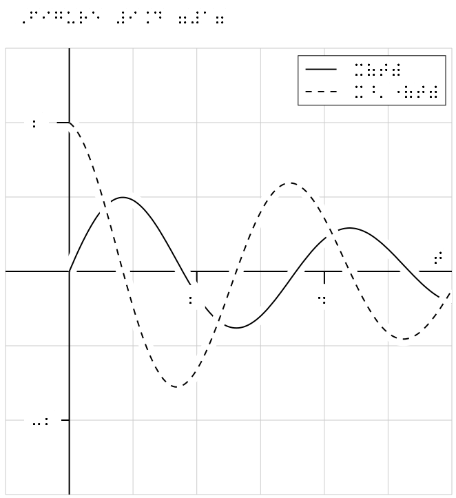
Subsection 10.3 LaTeX images
View Source for subsection
<subsection>
<title><latex/>
images</title>
<idx sortby="latex"><latex/>
image</idx>
<idx><h>image</h><h><latex/>
image</h></idx>
<p>
There are several graphics engine packages that a <latex/> document can employ.
Code from these packages renders diagrams automatically as part of normal processing of <latex/> files.
For HTML output the <c>pretext</c> script produces SVG versions of the pictures.
The script can also produce standalone <tex/> source files, PDFs, PNGs, and EPSs.
The packages should be loaded in <c>docinfo/latex-image-preamble</c>, which is also where global package settings should be made.
If any ampersands occur in your <latex/> code you should use the <c>\amp</c> macro pre-defined by <pretext/>.
These first examples are from the <url href="http://www.texample.net/tikz/examples/" visual="www.texample.net/tikz/examples/">TeXample.net</url> site.
Note that any <latex/> macros used in the rest of your document may be employed in the <latex/>-standalone or Asymptote diagrams (with this feature coming to Sage graphics next?).
</p>
<!-- http://www.texample.net/media/tikz/examples/TEX/noise-shaper.tex -->
<figure xml:id="figure-tikz-electronics">
<caption>TikZ Electronics Diagram</caption>
<image xml:id="tikz-electronics">
<shortdescription>
a pile of electronic components wired together
</shortdescription>
<latex-image>
<!-- CDATA prevents certain LaTeX code from being interpreted as xml -->
\tikzset{%
block/.style = {draw, thick, rectangle, minimum height = 3em,
minimum width = 3em},
sum/.style = {draw, circle, node distance = 2cm}, % Adder
input/.style = {coordinate}, % Input
output/.style = {coordinate} % Output
}
% Defining string as labels of certain blocks.
\newcommand{\suma}{\Large$+$}
\newcommand{\inte}{$\displaystyle \int$}
\newcommand{\derv}{\huge$\frac{d}{dt}$}
\begin{tikzpicture}[auto, thick, node distance=2cm, >=triangle 45]
\draw
% Drawing the blocks of first filter :
node at (0,0)[right=-3mm]{\Large \textbullet}
node [input, name=input1] {}
node [sum, right of=input1] (suma1) {\suma}
node [block, right of=suma1] (inte1) {\inte}
node at (6.8,0)[block] (Q1) {\Large $Q_1$}
node [block, below of=inte1] (ret1) {\Large$T_1$};
% Joining blocks.
% Commands \draw with options like [->] must be written individually
\draw[->](input1) -- node {$X(Z)$}(suma1);
\draw[->](suma1) -- node {} (inte1);
\draw[->](inte1) -- node {} (Q1);
\draw[->](ret1) -| node[near end]{} (suma1);
% Adder
\draw
node at (5.4,-4) [sum, name=suma2] {\suma}
% Second stage of filter
node at (1,-6) [sum, name=suma3] {\suma}
node [block, right of=suma3] (inte2) {\inte}
node [sum, right of=inte2] (suma4) {\suma}
node [block, right of=suma4] (inte3) {\inte}
node [block, right of=inte3] (Q2) {\Large$Q_2$}
node at (9,-8) [block, name=ret2] {\Large$T_2$}
;
% Joining the blocks of second filter
\draw[->] (suma3) -- node {} (inte2);
\draw[->] (inte2) -- node {} (suma4);
\draw[->] (suma4) -- node {} (inte3);
\draw[->] (inte3) -- node {} (Q2);
\draw[->] (ret2) -| (suma3);
\draw[->] (ret2) -| (suma4);
% Third stage of filter:
% Defining nodes:
\draw
node at (11.5, 0) [sum, name=suma5]{\suma}
node [output, right of=suma5]{}
node [block, below of=suma5] (deriv1){\derv}
node [output, right of=suma5] (sal2){}
;
% Joining the blocks:
\draw[->] (suma2) -| node {}(suma3);
\draw[->] (Q1) -- (8,0) |- node {}(ret1);
\draw[->] (8,0) |- (suma2);
\draw[->] (5.4,0) -- (suma2);
\draw[->] (Q1) -- node {}(suma5);
\draw[->] (deriv1) -- node {}(suma5);
\draw[->] (Q2) -| node {}(deriv1);
\draw[<->] (ret2) -| node {}(deriv1);
\draw[->] (suma5) -- node {$Y(Z)$}(sal2);
% Drawing nodes with \textbullet
\draw
node at (8,0) {\textbullet}
node at (8,-2){\textbullet}
node at (5.4,0){\textbullet}
node at (5,-8){\textbullet}
node at (11.5,-6){\textbullet}
;
% Boxing and labelling noise shapers
\draw [color=gray,thick](-0.5,-3) rectangle (9,1);
\node at (-0.5,1) [above=5mm, right=0mm] {\textsc{first-order noise shaper}};
\draw [color=gray,thick](-0.5,-9) rectangle (12.5,-5);
\node at (-0.5,-9) [below=5mm, right=0mm] {\textsc{second-order noise shaper}};
\end{tikzpicture}
</latex-image>
</image>
</figure>
<p>
The next example began life in <url href="http://www.frontiernet.net/~eugene.ressler/" visual="www.frontiernet.net/~eugene.ressler/">Sketch</url>, which will output TikZ code (though the code has been edited by hand for readability).
</p>
<!-- http://www.texample.net/media/tikz/examples/TEX/3d-cone.tex -->
<figure xml:id="figure-tikz-cone3D">
<caption>TikZ Cone Drawing</caption>
<image xml:id="tikz-cone" width="70%">
<latex-image>
<!-- CDATA prevents certain LaTeX code from being interpreted as xml -->
\begin{tikzpicture}[join=round]
\tikzstyle{conefill} = [fill=blue!20,fill opacity=0.8]
\tikzstyle{ann} = [fill=white,font=\footnotesize,inner sep=1pt]
\tikzstyle{ghostfill} = [fill=white]
\tikzstyle{ghostdraw} = [draw=black!50]
\filldraw[conefill](-.775,1.922)--(-1.162,.283)--(-.274,.5)
--(-.183,2.067)--cycle;
\filldraw[conefill](-.183,2.067)--(-.274,.5)--(.775,.424)
--(.516,2.016)--cycle;
\filldraw[conefill](.516,2.016)--(.775,.424)--(1.369,.1)
--(.913,1.8)--cycle;
\filldraw[conefill](-.913,1.667)--(-1.369,-.1)--(-1.162,.283)
--(-.775,1.922)--cycle;
\draw(1.461,.107)--(1.734,.127);
\draw[arrows=<->](1.643,1.853)--(1.643,.12);
\filldraw[conefill](.913,1.8)--(1.369,.1)--(1.162,-.283)
--(.775,1.545)--cycle;
\draw[arrows=->,line width=.4pt](.274,-.5)--(0,0)--(0,2.86);
\draw[arrows=-,line width=.4pt](0,0)--(-1.369,-.1);
\draw[arrows=->,line width=.4pt](-1.369,-.1)--(-2.1,-.153);
\filldraw[conefill](-.516,1.45)--(-.775,-.424)--(-1.369,-.1)
--(-.913,1.667)--cycle;
\draw(-1.369,.073)--(-1.369,2.76);
\draw(1.004,1.807)--(1.734,1.86);
\filldraw[conefill](.775,1.545)--(1.162,-.283)--(.274,-.5)
--(.183,1.4)--cycle;
\draw[arrows=<->](0,2.34)--(-.913,2.273);
\draw(-.913,1.84)--(-.913,2.447);
\draw[arrows=<->](0,2.687)--(-1.369,2.587);
\filldraw[conefill](.183,1.4)--(.274,-.5)--(-.775,-.424)
--(-.516,1.45)--cycle;
\draw[arrows=<-,line width=.4pt](.42,-.767)--(.274,-.5);
\node[ann] at (-.456,2.307) {$r_0$};
\node[ann] at (-.685,2.637) {$r_1$};
\node[ann] at (1.643,.987) {$h$};
\path (.42,-.767) node[below] {$x$}
(0,2.86) node[above] {$y$}
(-2.1,-.153) node[left] {$z$};
% Second version of the cone
\begin{scope}[xshift=3.5cm]
\filldraw[ghostdraw,ghostfill](-.775,1.922)--(-1.162,.283)--(-.274,.5)
--(-.183,2.067)--cycle;
\filldraw[ghostdraw,ghostfill](-.183,2.067)--(-.274,.5)--(.775,.424)
--(.516,2.016)--cycle;
\filldraw[ghostdraw,ghostfill](.516,2.016)--(.775,.424)--(1.369,.1)
--(.913,1.8)--cycle;
\filldraw[ghostdraw,ghostfill](-.913,1.667)--(-1.369,-.1)--(-1.162,.283)
--(-.775,1.922)--cycle;
\filldraw[ghostdraw,ghostfill](.913,1.8)--(1.369,.1)--(1.162,-.283)
--(.775,1.545)--cycle;
\filldraw[ghostdraw,ghostfill](-.516,1.45)--(-.775,-.424)--(-1.369,-.1)
--(-.913,1.667)--cycle;
\filldraw[ghostdraw,ghostfill](.775,1.545)--(1.162,-.283)--(.274,-.5)
--(.183,1.4)--cycle;
\filldraw[fill=red,fill opacity=0.5](-.516,1.45)--(-.775,-.424)--(.274,-.5)
--(.183,1.4)--cycle;
\fill(-.775,-.424) circle (2pt);
\fill(.274,-.5) circle (2pt);
\fill(-.516,1.45) circle (2pt);
\fill(.183,1.4) circle (2pt);
\path[font=\footnotesize]
(.913,1.8) node[right] {$i\hbox{$=$}0$}
(1.369,.1) node[right] {$i\hbox{$=$}1$};
\path[font=\footnotesize]
(-.645,.513) node[left] {$j$}
(.228,.45) node[right] {$j\hbox{$+$}1$};
\draw (-.209,.482)+(-60:.25) [yscale=1.3,->] arc(-60:240:.25);
\fill[black,font=\footnotesize]
(-.516,1.45) node [above] {$P_{00}$}
(-.775,-.424) node [below] {$P_{10}$}
(.183,1.4) node [above] {$P_{01}$}
(.274,-.5) node [below] {$P_{11}$};
\end{scope}
\end{tikzpicture}
</latex-image>
</image>
</figure>
<p>
The pgfplots package was included in <c>docinfo/latex-image-preamble</c>.
Here, it is used.
Also, here we demonstrate using <c>\amp</c> where you would normally use an ampersand in <latex/>.
There are known issues with <c>xelatex</c> processing any gradient shading in <c>tikz</c>.
To (successfully) create the gradient shading in the 3D image here, you may need to use <c>pdflatex</c> until <latex/> developers resolve this issue.
</p>
<figure xml:id="figure-pgfplots-demo">
<caption>Sample pgfplots plot</caption>
<image xml:id="pgfplots-demo">
<shortdescription>
a Cartesian plane with a function graph, a parametric curve, and some points
</shortdescription>
<latex-image>
<!-- CDATA prevents certain LaTeX code from being interpreted as xml -->
\begin{tikzpicture}
\matrix{
\begin{axis}[width = 0.5\linewidth]
\addplot[
domain = 0.1:10,
<->,
smooth,
thin,
color = blue,
]{4*ln(x)/ln(10)};
\addplot[
only marks,
]coordinates{
(0,2)
(4,3)
(2,4)
(3,4)};
\addplot[
variable = \t,
domain = 0:360,
samples = 200,
color = orange,
]({3*sin(2*t)}, {2*cos(5*t)});
\end{axis}
\amp
\begin{axis}[axis lines = box, width = 0.5\linewidth]
\addplot3[
surf,
faceted color = blue,
samples = 15,
domain = 0:1,
y domain = -1:1
]{x^2 - y^2};
\end{axis}\\
};
\end{tikzpicture}
</latex-image>
</image>
</figure>
<p>
A plot might use a graphics language to draw the axes and grid, but the data might be from an experiment and live in an external file that you do not wish to place in your source.
Place such a file in a subdirectory directly below the directory where your master source file resides.
Then indicate this directory in a <c>docinfo/directories/@data</c> attribute of your source.
But you <em>must</em> prefix the path with <c>data/</c> as in the source below.
</p>
<figure xml:id="figure-pgfplots-data-demo">

  <caption>External data in a pgfplots plot</caption>

  <image xml:id="pgfplots-data-demo">

    <shortdescription>
      a Cartesian plot of electric potential over time;
    </shortdescription>

    <latex-image>

    <!-- CDATA prevents certain LaTeX code from being interpreted as xml -->


  \begin{tikzpicture}
  \begin{axis}[
      xmin=0,xmax=100,ymin=-20,ymax=100,
      ytick={-20,0,...,100},
      xlabel={time (ms)},
      ylabel={potential (V)},
  ]
  \addplot[blue] table {data/dataplot/hodgkin-huxley-data.dat};
  \end{axis}
  \end{tikzpicture}
    </latex-image>

  </image>

</figure>
<p>
The TikZ image in the next figure is made up from two <init>PNG</init> images (the shark and the swimmer), in addition to various TikZ commands.
The images reside in a source directory, <c>numerical/attack</c>, so the image files (<c>shark.png</c>, <c>swimmer.png</c>) are prefixed in the TikZ code with <c>data/attack</c> so the creation of the image will be successful.
This example is courtesy of Stephen Brown.
</p>
<figure xml:id="figure-shark-attack">

  <caption>An illustration of the shark trying to catch you as you swim to shore.</caption>

  <image>

    <latex-image label="shark-attack">
  \begin{tikzpicture}
      \tikzset{ ragged border/.style={ decoration={random steps, segment length=1mm, amplitude=0.5mm}, decorate, } }
      \fill[cyan!30] decorate[ragged border]{ (0,2) -- (8,2) } -- (8,0) -- (0,0) -- cycle;
      \fill[yellow!30] decorate[ragged border]{ (8,2) -- (8,0) } -- (9,0) -- (9,2) -- cycle;
      \draw (1.5,1) node {\scalebox{-0.2}[0.2]{\includegraphics{data/attack/shark.png}}};
      \draw (5,1) node {\includegraphics[scale=0.05]{data/attack/swimmer.png}};
      \draw[|-|] (1.5,3) node [above] {\(\SI{0}{m}\)} -- (5,3) node [above] {\(\SI{50}{m}\)};
      \draw[|-|] (5,3) -- (8,3) node [above] {\(\SI{70}{m}\)};
  \end{tikzpicture}
    </latex-image>

  </image>

</figure>
<p>
A Cartesian plot might benefit from having a <tag>description</tag> with a <tag>tabular</tag> that lays bare the data used to to plot points.
</p>
<figure xml:id="figure-pgfplots-data-description">

  <caption>Full description with tabular</caption>

  <image width="70%">

    <shortdescription>
      a plot of some data points
    </shortdescription>

    <description>

      <p>
        A Cartesian graph plotting the following data.
      </p>

      <tabular row-headers="yes">

        <col right="minor"/> <col/><col/><col/> <col/><col/><col/> <col/><col/><col/>

        <row bottom="minor">

          <cell><m>x</m></cell>

          <cell><m>1</m></cell>

          <cell><m>2</m></cell>

          <cell><m>3</m></cell>

          <cell><m>4</m></cell>

          <cell><m>5</m></cell>

          <cell><m>6</m></cell>

          <cell><m>7</m></cell>

          <cell><m>8</m></cell>

          <cell><m>9</m></cell>

        </row>

        <row>

          <cell><m>y</m></cell>

          <cell><m>5</m></cell>

          <cell><m>3</m></cell>

          <cell><m>8</m></cell>

          <cell><m>9</m></cell>

          <cell><m>5</m></cell>

          <cell><m>5</m></cell>

          <cell><m>8</m></cell>

          <cell><m>2</m></cell>

          <cell><m>3</m></cell>

        </row>

      </tabular>

    </description>

    <latex-image label="pgfplots-data-description">
      \begin{tikzpicture}
          \begin{axis}[
                  xmin=0,
                  xmax=10,
                  ymin=-0,ymax=10,
                  xlabel={\(x\)},
                  ylabel={\(y\)},
              ]
              \addplot[only marks] coordinates {(1,5) (2,3) (3,8) (4,9) (5,5) (6,5) (7,8) (8,2) (9,3)};
          \end{axis}
      \end{tikzpicture}
    </latex-image>

  </image>

</figure>
<p>
The next image requires three passes with <latex/> to get everything in place.
It is placed here to test that the code in the Pythion script correctly recognizes this requirement.
</p>
<figure>

  <caption>A matrix with colored entries</caption>

  <!-- This image needs three passes with LaTeX, which --> <!-- is supported by the script making this image    -->

  <image width="50%">

    <latex-image label="latex-three-pass">
      \begin{tikzpicture}
      \node{
          $\begin{bNiceArray}{ccc|cc}[
          code-before={\cellcolor{green!72}{1-1,2-2,3-3}\cellcolor{teal!72}{1-2,2-3,3-4}\cellcolor{yellow!72}{1-3,2-4,3-5}}
          ]
          3 \amp 4 \amp 0 \amp 1 \amp 4 \\
          -2 \amp 3 \amp 1 \amp -2 \amp 3 \\
          0 \amp 2 \amp 1 \amp 0 \amp 2
          \end{bNiceArray}$
      };
  \end{tikzpicture}
    </latex-image>

  </image>

</figure>
<p>
PSTricks is a <latex/> package for drawing diagrams and pictures, dating back to the days before <init>PDF</init>, when PostScript (<init>PS</init>) was king.
Given its history, it does not seem to work easily with the <c>pdflatex</c> engine.
But it will work easily with the <c>xelatex</c> engine.
We try to keep this present sample document workable with both engines, so we have presented an example of the use of PSTricks in the <c>xelatex</c>-exclusive sample document where we test obscure fonts and characters.
So your best bet is to look there.
<idx>PSTricks</idx>
</p>
<p>
There are suggestions online that
<cd>\usepackage[pdf]{pstricks}</cd>
along with
<cd>pdflatex --shell-escape *.tex</cd>
is workable.
We could not make it happen, and a <q>shell escape</q> can be a dangerous security hole.
That said, updates to this approach are welcome.
</p>
</subsection>
There are several graphics engine packages that a LaTeX document can employ. Code from these packages renders diagrams automatically as part of normal processing of LaTeX files. For HTML output the
pretext script produces SVG versions of the pictures. The script can also produce standalone TeX source files, PDFs, PNGs, and EPSs. The packages should be loaded in docinfo/latex-image-preamble, which is also where global package settings should be made. If any ampersands occur in your LaTeX code you should use the \amp macro pre-defined by PreTeXt. These first examples are from the TeXample.net site. Note that any LaTeX macros used in the rest of your document may be employed in the LaTeX-standalone or Asymptote diagrams (with this feature coming to Sage graphics next?).
View Source for figure
<figure xml:id="figure-tikz-electronics">
<caption>TikZ Electronics Diagram</caption>
<image xml:id="tikz-electronics">
<shortdescription>
a pile of electronic components wired together
</shortdescription>
<latex-image>
<!-- CDATA prevents certain LaTeX code from being interpreted as xml -->
\tikzset{%
block/.style = {draw, thick, rectangle, minimum height = 3em,
minimum width = 3em},
sum/.style = {draw, circle, node distance = 2cm}, % Adder
input/.style = {coordinate}, % Input
output/.style = {coordinate} % Output
}
% Defining string as labels of certain blocks.
\newcommand{\suma}{\Large$+$}
\newcommand{\inte}{$\displaystyle \int$}
\newcommand{\derv}{\huge$\frac{d}{dt}$}
\begin{tikzpicture}[auto, thick, node distance=2cm, >=triangle 45]
\draw
% Drawing the blocks of first filter :
node at (0,0)[right=-3mm]{\Large \textbullet}
node [input, name=input1] {}
node [sum, right of=input1] (suma1) {\suma}
node [block, right of=suma1] (inte1) {\inte}
node at (6.8,0)[block] (Q1) {\Large $Q_1$}
node [block, below of=inte1] (ret1) {\Large$T_1$};
% Joining blocks.
% Commands \draw with options like [->] must be written individually
\draw[->](input1) -- node {$X(Z)$}(suma1);
\draw[->](suma1) -- node {} (inte1);
\draw[->](inte1) -- node {} (Q1);
\draw[->](ret1) -| node[near end]{} (suma1);
% Adder
\draw
node at (5.4,-4) [sum, name=suma2] {\suma}
% Second stage of filter
node at (1,-6) [sum, name=suma3] {\suma}
node [block, right of=suma3] (inte2) {\inte}
node [sum, right of=inte2] (suma4) {\suma}
node [block, right of=suma4] (inte3) {\inte}
node [block, right of=inte3] (Q2) {\Large$Q_2$}
node at (9,-8) [block, name=ret2] {\Large$T_2$}
;
% Joining the blocks of second filter
\draw[->] (suma3) -- node {} (inte2);
\draw[->] (inte2) -- node {} (suma4);
\draw[->] (suma4) -- node {} (inte3);
\draw[->] (inte3) -- node {} (Q2);
\draw[->] (ret2) -| (suma3);
\draw[->] (ret2) -| (suma4);
% Third stage of filter:
% Defining nodes:
\draw
node at (11.5, 0) [sum, name=suma5]{\suma}
node [output, right of=suma5]{}
node [block, below of=suma5] (deriv1){\derv}
node [output, right of=suma5] (sal2){}
;
% Joining the blocks:
\draw[->] (suma2) -| node {}(suma3);
\draw[->] (Q1) -- (8,0) |- node {}(ret1);
\draw[->] (8,0) |- (suma2);
\draw[->] (5.4,0) -- (suma2);
\draw[->] (Q1) -- node {}(suma5);
\draw[->] (deriv1) -- node {}(suma5);
\draw[->] (Q2) -| node {}(deriv1);
\draw[<->] (ret2) -| node {}(deriv1);
\draw[->] (suma5) -- node {$Y(Z)$}(sal2);
% Drawing nodes with \textbullet
\draw
node at (8,0) {\textbullet}
node at (8,-2){\textbullet}
node at (5.4,0){\textbullet}
node at (5,-8){\textbullet}
node at (11.5,-6){\textbullet}
;
% Boxing and labelling noise shapers
\draw [color=gray,thick](-0.5,-3) rectangle (9,1);
\node at (-0.5,1) [above=5mm, right=0mm] {\textsc{first-order noise shaper}};
\draw [color=gray,thick](-0.5,-9) rectangle (12.5,-5);
\node at (-0.5,-9) [below=5mm, right=0mm] {\textsc{second-order noise shaper}};
\end{tikzpicture}
</latex-image>
</image>
</figure>

The next example began life in Sketch, which will output TikZ code (though the code has been edited by hand for readability).
View Source for figure
<figure xml:id="figure-tikz-cone3D">
<caption>TikZ Cone Drawing</caption>
<image xml:id="tikz-cone" width="70%">
<latex-image>
<!-- CDATA prevents certain LaTeX code from being interpreted as xml -->
\begin{tikzpicture}[join=round]
\tikzstyle{conefill} = [fill=blue!20,fill opacity=0.8]
\tikzstyle{ann} = [fill=white,font=\footnotesize,inner sep=1pt]
\tikzstyle{ghostfill} = [fill=white]
\tikzstyle{ghostdraw} = [draw=black!50]
\filldraw[conefill](-.775,1.922)--(-1.162,.283)--(-.274,.5)
--(-.183,2.067)--cycle;
\filldraw[conefill](-.183,2.067)--(-.274,.5)--(.775,.424)
--(.516,2.016)--cycle;
\filldraw[conefill](.516,2.016)--(.775,.424)--(1.369,.1)
--(.913,1.8)--cycle;
\filldraw[conefill](-.913,1.667)--(-1.369,-.1)--(-1.162,.283)
--(-.775,1.922)--cycle;
\draw(1.461,.107)--(1.734,.127);
\draw[arrows=<->](1.643,1.853)--(1.643,.12);
\filldraw[conefill](.913,1.8)--(1.369,.1)--(1.162,-.283)
--(.775,1.545)--cycle;
\draw[arrows=->,line width=.4pt](.274,-.5)--(0,0)--(0,2.86);
\draw[arrows=-,line width=.4pt](0,0)--(-1.369,-.1);
\draw[arrows=->,line width=.4pt](-1.369,-.1)--(-2.1,-.153);
\filldraw[conefill](-.516,1.45)--(-.775,-.424)--(-1.369,-.1)
--(-.913,1.667)--cycle;
\draw(-1.369,.073)--(-1.369,2.76);
\draw(1.004,1.807)--(1.734,1.86);
\filldraw[conefill](.775,1.545)--(1.162,-.283)--(.274,-.5)
--(.183,1.4)--cycle;
\draw[arrows=<->](0,2.34)--(-.913,2.273);
\draw(-.913,1.84)--(-.913,2.447);
\draw[arrows=<->](0,2.687)--(-1.369,2.587);
\filldraw[conefill](.183,1.4)--(.274,-.5)--(-.775,-.424)
--(-.516,1.45)--cycle;
\draw[arrows=<-,line width=.4pt](.42,-.767)--(.274,-.5);
\node[ann] at (-.456,2.307) {$r_0$};
\node[ann] at (-.685,2.637) {$r_1$};
\node[ann] at (1.643,.987) {$h$};
\path (.42,-.767) node[below] {$x$}
(0,2.86) node[above] {$y$}
(-2.1,-.153) node[left] {$z$};
% Second version of the cone
\begin{scope}[xshift=3.5cm]
\filldraw[ghostdraw,ghostfill](-.775,1.922)--(-1.162,.283)--(-.274,.5)
--(-.183,2.067)--cycle;
\filldraw[ghostdraw,ghostfill](-.183,2.067)--(-.274,.5)--(.775,.424)
--(.516,2.016)--cycle;
\filldraw[ghostdraw,ghostfill](.516,2.016)--(.775,.424)--(1.369,.1)
--(.913,1.8)--cycle;
\filldraw[ghostdraw,ghostfill](-.913,1.667)--(-1.369,-.1)--(-1.162,.283)
--(-.775,1.922)--cycle;
\filldraw[ghostdraw,ghostfill](.913,1.8)--(1.369,.1)--(1.162,-.283)
--(.775,1.545)--cycle;
\filldraw[ghostdraw,ghostfill](-.516,1.45)--(-.775,-.424)--(-1.369,-.1)
--(-.913,1.667)--cycle;
\filldraw[ghostdraw,ghostfill](.775,1.545)--(1.162,-.283)--(.274,-.5)
--(.183,1.4)--cycle;
\filldraw[fill=red,fill opacity=0.5](-.516,1.45)--(-.775,-.424)--(.274,-.5)
--(.183,1.4)--cycle;
\fill(-.775,-.424) circle (2pt);
\fill(.274,-.5) circle (2pt);
\fill(-.516,1.45) circle (2pt);
\fill(.183,1.4) circle (2pt);
\path[font=\footnotesize]
(.913,1.8) node[right] {$i\hbox{$=$}0$}
(1.369,.1) node[right] {$i\hbox{$=$}1$};
\path[font=\footnotesize]
(-.645,.513) node[left] {$j$}
(.228,.45) node[right] {$j\hbox{$+$}1$};
\draw (-.209,.482)+(-60:.25) [yscale=1.3,->] arc(-60:240:.25);
\fill[black,font=\footnotesize]
(-.516,1.45) node [above] {$P_{00}$}
(-.775,-.424) node [below] {$P_{10}$}
(.183,1.4) node [above] {$P_{01}$}
(.274,-.5) node [below] {$P_{11}$};
\end{scope}
\end{tikzpicture}
</latex-image>
</image>
</figure>

The pgfplots package was included in
docinfo/latex-image-preamble. Here, it is used. Also, here we demonstrate using \amp where you would normally use an ampersand in LaTeX. There are known issues with xelatex processing any gradient shading in tikz. To (successfully) create the gradient shading in the 3D image here, you may need to use pdflatex until LaTeX developers resolve this issue.
View Source for figure
<figure xml:id="figure-pgfplots-demo">
<caption>Sample pgfplots plot</caption>
<image xml:id="pgfplots-demo">
<shortdescription>
a Cartesian plane with a function graph, a parametric curve, and some points
</shortdescription>
<latex-image>
<!-- CDATA prevents certain LaTeX code from being interpreted as xml -->
\begin{tikzpicture}
\matrix{
\begin{axis}[width = 0.5\linewidth]
\addplot[
domain = 0.1:10,
<->,
smooth,
thin,
color = blue,
]{4*ln(x)/ln(10)};
\addplot[
only marks,
]coordinates{
(0,2)
(4,3)
(2,4)
(3,4)};
\addplot[
variable = \t,
domain = 0:360,
samples = 200,
color = orange,
]({3*sin(2*t)}, {2*cos(5*t)});
\end{axis}
\amp
\begin{axis}[axis lines = box, width = 0.5\linewidth]
\addplot3[
surf,
faceted color = blue,
samples = 15,
domain = 0:1,
y domain = -1:1
]{x^2 - y^2};
\end{axis}\\
};
\end{tikzpicture}
</latex-image>
</image>
</figure>

A plot might use a graphics language to draw the axes and grid, but the data might be from an experiment and live in an external file that you do not wish to place in your source. Place such a file in a subdirectory directly below the directory where your master source file resides. Then indicate this directory in a
docinfo/directories/@data attribute of your source. But you must prefix the path with data/ as in the source below.
View Source for figure
<figure xml:id="figure-pgfplots-data-demo">
<caption>External data in a pgfplots plot</caption>
<image xml:id="pgfplots-data-demo">
<shortdescription>
a Cartesian plot of electric potential over time;
</shortdescription>
<latex-image>
<!-- CDATA prevents certain LaTeX code from being interpreted as xml -->
\begin{tikzpicture}
\begin{axis}[
xmin=0,xmax=100,ymin=-20,ymax=100,
ytick={-20,0,...,100},
xlabel={time (ms)},
ylabel={potential (V)},
]
\addplot[blue] table {data/dataplot/hodgkin-huxley-data.dat};
\end{axis}
\end{tikzpicture}
</latex-image>
</image>
</figure>

The TikZ image in the next figure is made up from two PNG images (the shark and the swimmer), in addition to various TikZ commands. The images reside in a source directory,
numerical/attack, so the image files (shark.png, swimmer.png) are prefixed in the TikZ code with data/attack so the creation of the image will be successful. This example is courtesy of Stephen Brown.
View Source for figure
<figure xml:id="figure-shark-attack">
<caption>An illustration of the shark trying to catch you as you swim to shore.</caption>
<image>
<latex-image label="shark-attack">
\begin{tikzpicture}
\tikzset{ ragged border/.style={ decoration={random steps, segment length=1mm, amplitude=0.5mm}, decorate, } }
\fill[cyan!30] decorate[ragged border]{ (0,2) -- (8,2) } -- (8,0) -- (0,0) -- cycle;
\fill[yellow!30] decorate[ragged border]{ (8,2) -- (8,0) } -- (9,0) -- (9,2) -- cycle;
\draw (1.5,1) node {\scalebox{-0.2}[0.2]{\includegraphics{data/attack/shark.png}}};
\draw (5,1) node {\includegraphics[scale=0.05]{data/attack/swimmer.png}};
\draw[|-|] (1.5,3) node [above] {\(\SI{0}{m}\)} -- (5,3) node [above] {\(\SI{50}{m}\)};
\draw[|-|] (5,3) -- (8,3) node [above] {\(\SI{70}{m}\)};
\end{tikzpicture}
</latex-image>
</image>
</figure>

A Cartesian plot might benefit from having a
<description> with a <tabular> that lays bare the data used to to plot points.
View Source for figure
<figure xml:id="figure-pgfplots-data-description">
<caption>Full description with tabular</caption>
<image width="70%">
<shortdescription>
a plot of some data points
</shortdescription>
<description>
<p>
A Cartesian graph plotting the following data.
</p>
<tabular row-headers="yes">
<col right="minor"/> <col/><col/><col/> <col/><col/><col/> <col/><col/><col/>
<row bottom="minor">
<cell><m>x</m></cell>
<cell><m>1</m></cell>
<cell><m>2</m></cell>
<cell><m>3</m></cell>
<cell><m>4</m></cell>
<cell><m>5</m></cell>
<cell><m>6</m></cell>
<cell><m>7</m></cell>
<cell><m>8</m></cell>
<cell><m>9</m></cell>
</row>
<row>
<cell><m>y</m></cell>
<cell><m>5</m></cell>
<cell><m>3</m></cell>
<cell><m>8</m></cell>
<cell><m>9</m></cell>
<cell><m>5</m></cell>
<cell><m>5</m></cell>
<cell><m>8</m></cell>
<cell><m>2</m></cell>
<cell><m>3</m></cell>
</row>
</tabular>
</description>
<latex-image label="pgfplots-data-description">
\begin{tikzpicture}
\begin{axis}[
xmin=0,
xmax=10,
ymin=-0,ymax=10,
xlabel={\(x\)},
ylabel={\(y\)},
]
\addplot[only marks] coordinates {(1,5) (2,3) (3,8) (4,9) (5,5) (6,5) (7,8) (8,2) (9,3)};
\end{axis}
\end{tikzpicture}
</latex-image>
</image>
</figure>

A Cartesian graph plotting the following data.
| \(x\) | \(1\) | \(2\) | \(3\) | \(4\) | \(5\) | \(6\) | \(7\) | \(8\) | \(9\) |
|---|---|---|---|---|---|---|---|---|---|
| \(y\) | \(5\) | \(3\) | \(8\) | \(9\) | \(5\) | \(5\) | \(8\) | \(2\) | \(3\) |
The next image requires three passes with LaTeX to get everything in place. It is placed here to test that the code in the Pythion script correctly recognizes this requirement.
View Source for figure
<figure>
<caption>A matrix with colored entries</caption>
<!-- This image needs three passes with LaTeX, which --> <!-- is supported by the script making this image -->
<image width="50%">
<latex-image label="latex-three-pass">
\begin{tikzpicture}
\node{
$\begin{bNiceArray}{ccc|cc}[
code-before={\cellcolor{green!72}{1-1,2-2,3-3}\cellcolor{teal!72}{1-2,2-3,3-4}\cellcolor{yellow!72}{1-3,2-4,3-5}}
]
3 \amp 4 \amp 0 \amp 1 \amp 4 \\
-2 \amp 3 \amp 1 \amp -2 \amp 3 \\
0 \amp 2 \amp 1 \amp 0 \amp 2
\end{bNiceArray}$
};
\end{tikzpicture}
</latex-image>
</image>
</figure>

PSTricks is a LaTeX package for drawing diagrams and pictures, dating back to the days before PDF, when PostScript (PS) was king. Given its history, it does not seem to work easily with the
pdflatex engine. But it will work easily with the xelatex engine. We try to keep this present sample document workable with both engines, so we have presented an example of the use of PSTricks in the xelatex-exclusive sample document where we test obscure fonts and characters. So your best bet is to look there.
There are suggestions online that
\usepackage[pdf]{pstricks}
along with
pdflatex --shell-escape *.tex
is workable. We could not make it happen, and a “shell escape” can be a dangerous security hole. That said, updates to this approach are welcome.
Subsection 10.4 Asymptote, 2D
View Source for subsection
<subsection>

  <title>Asymptote, 2D</title>

  <p>
    The Asymptote
    <idx><h>asymptote graphics language</h></idx>
    graphics language may be placed in your source to draw graphs, diagrams or pictures.
    Rules for formatting code are identical to those for Sage code.
    For more on Asymptote see <url href="http://asymptote.sourceforge.net/" visual="asymptote.sourceforge.net"/>.
  </p>

  <!-- See a different (more traditional) variant of URL usage in the introductory section. -->

  <p>
    This is a simple physics diagram about levers, taken from the Asymptote documentation.
    In the HTML version of this article, the images are SVG's and so should scale nicely when you zoom in on the page.
  </p>

  <!-- http://asymptote.sourceforge.net/gallery/lever.asy --> <!-- xml:id's on the figures may be employed for cross-references, while the xml:id's on the actual graphics code will be used to name the files that are created.  They are optional, in which case, generic names will be created, though these use serial numbers and so will change as more are added. -->

  <figure xml:id="figure-asymptote-levers">

    <caption>Asymptote Lever Demonstration</caption>

    <image xml:id="asymptote-lever">

      <shortdescription>
        moments on a lever
      </shortdescription>

      <description>

        <p>
          This diagram has two masses at either end of a lever, namely <m>m</m> and <m>M</m>.
          They are located at distance <m>x</m> and <m>X</m> on an axis.
          The resulting center-of-mass is at a point <m>\bar{x}</m>.
        </p>

      </description>

      <asymptote>
    size(200,0);
    pair z0=(0,0);
    pair z1=(2,0);
    pair z2=(5,0);
    pair zf=z1+0.75*(z2-z1);
    draw(z1--z2);
    dot(z1,red+0.15cm);
    dot(z2,darkgreen+0.3cm);
    label("$m$",z1,1.2N,red);
    label("$M$",z2,1.5N,darkgreen);
    label("$\hat{\ }$",zf,0.2*S,fontsize(24pt)+blue);
    pair s=-0.2*I;
    draw("$x$",z0+s--z1+s,N,red,Arrows,Bars,PenMargins);
    s=-0.5*I;
    draw("$\bar{x}$",z0+s--zf+s,blue,Arrows,Bars,PenMargins);
    s=-0.95*I;
    draw("$X$",z0+s--z2+s,darkgreen,Arrows,Bars,PenMargins);
      </asymptote>

    </image>

  </figure>

  <p>
    And a colorful contour plot with logarithmic scale.
    Again, from the Asymptote documentation.
    This SVG image employs two additional PNG images for the two parts where the color varies continuously.
  </p>

  <!-- http://asymptote.sourceforge.net/gallery/2D%20graphs/logimage.asy -->

  <figure xml:id="figure-asymptote-contour-plot">

    <caption>Asymptote Contour Plot</caption>

    <image xml:id="asymptote-contour">

      <asymptote>
    import graph;
    import palette;
    size(10cm,10cm,IgnoreAspect);
    real f(real x, real y) {
      return 0.9*pow10(2*sin(x/5+2*y^0.25)) + 0.1*(1+cos(10*log(y)));
    }
    scale(Linear,Log,Log);
    pen[] Palette=BWRainbow();
    bounds range=image(f,Automatic,(0,1),(100,100),nx=200,Palette);
    xaxis("$x$",BottomTop,LeftTicks,above=true);
    yaxis("$y$",LeftRight,RightTicks,above=true);
    palette("$f(x,y)$",range,(0,200),(100,250),Top,Palette,
            PaletteTicks(ptick=linewidth(0.5*linewidth())));
      </asymptote>

    </image>

  </figure>

  <p>
    Here is the lever diagram again, but now we have added an integral to one of the legends, <em>using a <latex/> macro of our own,</em> which is idential to one we used in the early part of this article.
    The point is, we only needed to define the macro once for the entire document, and it is available as we make Asymptote diagrams.
    This device can be used to maintain flexibility and consistency in your choice of notation.
  </p>

  <figure xml:id="figure-asymptote-latex-macro">

    <caption>Aymptote Lever, plus Integral</caption>

    <image xml:id="asymptote-lever-integral" width="80%">

      <asymptote>
    size(200,0);
    pair z0=(0,0);
    pair z1=(2,0);
    pair z2=(5,0);
    pair zf=z1+0.75*(z2-z1);
    draw(z1--z2);
    dot(z1,red+0.15cm);
    dot(z2,darkgreen+0.3cm);
    label("$m$",z1,1.2N,red);
    label("$M$",z2,1.5N,darkgreen);
    label("$\hat{\ }$",zf,0.2*S,fontsize(24pt)+blue);
    pair s=-0.2*I;
    draw("$x$",z0+s--z1+s,N,red,Arrows,Bars,PenMargins);
    s=-0.5*I;
    draw("$\bar{x}=\definiteintegral{0}{1}{x\delta(x)}{x}$",z0+s--zf+s,blue,Arrows,Bars,PenMargins);
    s=-1.05*I;
    draw("$X$",z0+s--z2+s,darkgreen,Arrows,Bars,PenMargins);
      </asymptote>

    </image>

  </figure>

</subsection>
The Asymptote graphics language may be placed in your source to draw graphs, diagrams or pictures. Rules for formatting code are identical to those for Sage code. For more on Asymptote see
asymptote.sourceforge.net.
This is a simple physics diagram about levers, taken from the Asymptote documentation. In the HTML version of this article, the images are SVG’s and so should scale nicely when you zoom in on the page.
View Source for figure
<figure xml:id="figure-asymptote-levers">

  <caption>Asymptote Lever Demonstration</caption>

  <image xml:id="asymptote-lever">

    <shortdescription>
      moments on a lever
    </shortdescription>

    <description>

      <p>
        This diagram has two masses at either end of a lever, namely <m>m</m> and <m>M</m>.
        They are located at distance <m>x</m> and <m>X</m> on an axis.
        The resulting center-of-mass is at a point <m>\bar{x}</m>.
      </p>

    </description>

    <asymptote>
  size(200,0);
  pair z0=(0,0);
  pair z1=(2,0);
  pair z2=(5,0);
  pair zf=z1+0.75*(z2-z1);
  draw(z1--z2);
  dot(z1,red+0.15cm);
  dot(z2,darkgreen+0.3cm);
  label("$m$",z1,1.2N,red);
  label("$M$",z2,1.5N,darkgreen);
  label("$\hat{\ }$",zf,0.2*S,fontsize(24pt)+blue);
  pair s=-0.2*I;
  draw("$x$",z0+s--z1+s,N,red,Arrows,Bars,PenMargins);
  s=-0.5*I;
  draw("$\bar{x}$",z0+s--zf+s,blue,Arrows,Bars,PenMargins);
  s=-0.95*I;
  draw("$X$",z0+s--z2+s,darkgreen,Arrows,Bars,PenMargins);
    </asymptote>

  </image>

</figure>
This diagram has two masses at either end of a lever, namely \(m\) and \(M\text{.}\) They are located at distance \(x\) and \(X\) on an axis. The resulting center-of-mass is at a point \(\bar{x}\text{.}\)
And a colorful contour plot with logarithmic scale. Again, from the Asymptote documentation. This SVG image employs two additional PNG images for the two parts where the color varies continuously.
View Source for figure
<figure xml:id="figure-asymptote-contour-plot">

  <caption>Asymptote Contour Plot</caption>

  <image xml:id="asymptote-contour">

    <asymptote>
  import graph;
  import palette;
  size(10cm,10cm,IgnoreAspect);
  real f(real x, real y) {
    return 0.9*pow10(2*sin(x/5+2*y^0.25)) + 0.1*(1+cos(10*log(y)));
  }
  scale(Linear,Log,Log);
  pen[] Palette=BWRainbow();
  bounds range=image(f,Automatic,(0,1),(100,100),nx=200,Palette);
  xaxis("$x$",BottomTop,LeftTicks,above=true);
  yaxis("$y$",LeftRight,RightTicks,above=true);
  palette("$f(x,y)$",range,(0,200),(100,250),Top,Palette,
          PaletteTicks(ptick=linewidth(0.5*linewidth())));
    </asymptote>

  </image>

</figure>
Here is the lever diagram again, but now we have added an integral to one of the legends, using a LaTeX macro of our own, which is idential to one we used in the early part of this article. The point is, we only needed to define the macro once for the entire document, and it is available as we make Asymptote diagrams. This device can be used to maintain flexibility and consistency in your choice of notation.
View Source for figure
<figure xml:id="figure-asymptote-latex-macro">

  <caption>Aymptote Lever, plus Integral</caption>

  <image xml:id="asymptote-lever-integral" width="80%">

    <asymptote>
  size(200,0);
  pair z0=(0,0);
  pair z1=(2,0);
  pair z2=(5,0);
  pair zf=z1+0.75*(z2-z1);
  draw(z1--z2);
  dot(z1,red+0.15cm);
  dot(z2,darkgreen+0.3cm);
  label("$m$",z1,1.2N,red);
  label("$M$",z2,1.5N,darkgreen);
  label("$\hat{\ }$",zf,0.2*S,fontsize(24pt)+blue);
  pair s=-0.2*I;
  draw("$x$",z0+s--z1+s,N,red,Arrows,Bars,PenMargins);
  s=-0.5*I;
  draw("$\bar{x}=\definiteintegral{0}{1}{x\delta(x)}{x}$",z0+s--zf+s,blue,Arrows,Bars,PenMargins);
  s=-1.05*I;
  draw("$X$",z0+s--z2+s,darkgreen,Arrows,Bars,PenMargins);
    </asymptote>

  </image>

</figure>
Subsection 10.5 Asymptote, 3D via WebGL
View Source for subsection
<subsection xml:id="graphics-asymptote-webgl">

  <title>Asymptote, 3D via WebGL</title>

  <p>
    Asymptote can create an <init>HTML</init> file that is an interactive version of a 3D shape.
    At this writing (2020-05-18) support via the <c>pretext</c> script is evolving.
    Plus, you will need newer versions of Asymptote and the <c>dvisvgm</c> utility to duplicate all of the results being displayed here in this testing document.
    The other distinction is that the author needs to provide the aspect ratio of the figure, and this should be placed on the <tag>asymptote</tag> element (not on the <tag>image</tag> element).
    <xref ref="figure-asymptote-workcone"/> is from the <url href="http://asymptote.sourceforge.net/gallery/3Dwebgl/" visual="asymptote.sourceforge.net/gallery/3Dwebgl/">Asymptote Gallery</url>.
  </p>

  <figure xml:id="figure-asymptote-workcone">

    <caption>Work Cone (Asymptote Interactive 3D Image)</caption>

    <image xml:id="asymptote-workcone" width="50%">

      <asymptote>
    import solids;
    size(0,150);
    currentprojection=orthographic(0,-30,5);
    real r=4;
    real h=10;
    real s=8;
    real x=r*s/h;
    real sr=5;
    real xr=r*sr/h;
    real s1=sr-0.1;
    real x1=r*s1/h;
    real s2=sr+0.2;
    real x2=r*s2/h;
    render render=render(compression=0,merge=true);
    draw(scale(x1,x1,-s1)*shift(-Z)*unitcone,lightblue+opacity(0.5),render);
    path3 p=(x2,0,s2)--(x,0,s+0.005);
    revolution a=revolution(p,Z);
    draw(surface(a),lightblue+opacity(0.5),render);
    path3 q=(x,0,s)--(r,0,h);
    revolution b=revolution(q,Z);
    draw(surface(b),white+opacity(0.5),render);
    draw((-r-1,0,0)--(r+1,0,0));
    draw((0,0,0)--(0,0,h+1),dashed);
    path3 w=(x1,0,s1)--(x2,0,s2)--(0,0,s2);
    revolution b=revolution(w,Z);
    draw(surface(b),blue+opacity(0.5),render);
    draw(circle((0,0,s2),x2));
    draw(circle((0,0,s1),x1));
    draw("$x$",(xr,0,0)--(xr,0,sr),red,Arrow3,PenMargin3);
    draw("$r$",(0,0,sr)--(xr,0,sr),N,red);
    draw((string) r,(0,0,h)--(r,0,h),N,red);
    draw((string) h,(r,0,0)--(r,0,h),red,Arrow3,PenMargin3);
    draw((string) s,(-x,0,0)--(-x,0,s),W,red,Arrow3,Bar3,PenMargin3);
      </asymptote>

    </image>

  </figure>

  <p>
    These 3D images in HTML output are rotable with a pointing device (mouse, trackpad) with a click-and-drag.
    A finger should suffice on touch-sensitive devices (phones, tablets).
    Zooming in and out can be accomplished with a mouse wheel, or by pinching.
    As a contribution to the accessibility of <pretext/> HTML output, keyboard controls will also allow for exploration of these images.
    (Make sure the image has focus when you attempt to use these.)
  </p>

  <!-- More possible keyboard shortcuts are at Section 8.29, page 136 --> <!-- https://asymptote.sourceforge.io/asymptote.pdf                 --> <!-- Not all seem to be implented, so review/test carefully         -->

  <table>

    <title>3D Image Keyboard Controls</title>

    <tabular>

      <row bottom="medium">

        <cell>Key</cell>

        <cell>Action</cell>

      </row>

      <row>

        <cell><kbd>x</kbd></cell>

        <cell>Rotate around <m>x</m>-axis</cell>

      </row>

      <row>

        <cell><kbd>y</kbd></cell>

        <cell>Rotate around <m>y</m>-axis</cell>

      </row>

      <row>

        <cell><kbd>z</kbd></cell>

        <cell>Rotate around <m>z</m>-axis</cell>

      </row>

      <row>

        <cell><kbd>+</kbd></cell>

        <cell>Enlarge image</cell>

      </row>

      <row>

        <cell><kbd>-</kbd></cell>

        <cell>Shrink image</cell>

      </row>

      <row>

        <cell><kbd>h</kbd></cell>

        <cell>Return to home position</cell>

      </row>

    </tabular>

  </table>

  <p>
    And finally, an example of a 3-D graph (from the Asymptote documentation again).
    This WebGL image is a beautiful example of a Riemann surface.
    As you rotate the image, notice how the reflection of the light source varies, along with the brightness of various regions of the surface.
    This example is accomplished with just 10 lines of Asymptote code.
  </p>

  <!-- http://asymptote.sourceforge.net/gallery/3D%20graphs/filesurface.asy --> <!-- Projection point adjusted by Michael Doob -->

  <figure xml:id="figure-asymptote-surface">

    <caption>Asymptote 3-D Surface</caption>

    <image xml:id="asymptote-surface" width="40%">

      <asymptote>
    // Riemann surface of z^{1/n}
    import graph3;
    import palette;
    int n=3;
    size(200,300,keepAspect=false);
    currentprojection=orthographic(10,10,5);
    currentlight=(10,10,5);
    triple f(pair t) {return (t.x*cos(t.y),t.x*sin(t.y),t.x^(1/n)*sin(t.y/n));}
    surface s=surface(f,(0,0),(1,2pi*n),8,16,Spline);
    s.colors(palette(s.map(zpart),Rainbow()));
    draw(s,meshpen=black,render(merge=true));
      </asymptote>

    </image>

  </figure>

</subsection>
Asymptote can create an HTML file that is an interactive version of a 3D shape. At this writing (2020-05-18) support via the
pretext script is evolving. Plus, you will need newer versions of Asymptote and the dvisvgm utility to duplicate all of the results being displayed here in this testing document. The other distinction is that the author needs to provide the aspect ratio of the figure, and this should be placed on the <asymptote> element (not on the <image> element). Figure 10.16 is from the Asymptote Gallery.
View Source for figure
<figure xml:id="figure-asymptote-workcone">

  <caption>Work Cone (Asymptote Interactive 3D Image)</caption>

  <image xml:id="asymptote-workcone" width="50%">

    <asymptote>
  import solids;
  size(0,150);
  currentprojection=orthographic(0,-30,5);
  real r=4;
  real h=10;
  real s=8;
  real x=r*s/h;
  real sr=5;
  real xr=r*sr/h;
  real s1=sr-0.1;
  real x1=r*s1/h;
  real s2=sr+0.2;
  real x2=r*s2/h;
  render render=render(compression=0,merge=true);
  draw(scale(x1,x1,-s1)*shift(-Z)*unitcone,lightblue+opacity(0.5),render);
  path3 p=(x2,0,s2)--(x,0,s+0.005);
  revolution a=revolution(p,Z);
  draw(surface(a),lightblue+opacity(0.5),render);
  path3 q=(x,0,s)--(r,0,h);
  revolution b=revolution(q,Z);
  draw(surface(b),white+opacity(0.5),render);
  draw((-r-1,0,0)--(r+1,0,0));
  draw((0,0,0)--(0,0,h+1),dashed);
  path3 w=(x1,0,s1)--(x2,0,s2)--(0,0,s2);
  revolution b=revolution(w,Z);
  draw(surface(b),blue+opacity(0.5),render);
  draw(circle((0,0,s2),x2));
  draw(circle((0,0,s1),x1));
  draw("$x$",(xr,0,0)--(xr,0,sr),red,Arrow3,PenMargin3);
  draw("$r$",(0,0,sr)--(xr,0,sr),N,red);
  draw((string) r,(0,0,h)--(r,0,h),N,red);
  draw((string) h,(r,0,0)--(r,0,h),red,Arrow3,PenMargin3);
  draw((string) s,(-x,0,0)--(-x,0,s),W,red,Arrow3,Bar3,PenMargin3);
    </asymptote>

  </image>

</figure>
These 3D images in HTML output are rotable with a pointing device (mouse, trackpad) with a click-and-drag. A finger should suffice on touch-sensitive devices (phones, tablets). Zooming in and out can be accomplished with a mouse wheel, or by pinching. As a contribution to the accessibility of PreTeXt HTML output, keyboard controls will also allow for exploration of these images. (Make sure the image has focus when you attempt to use these.)
View Source for table
<table>

  <title>3D Image Keyboard Controls</title>

  <tabular>

    <row bottom="medium">

      <cell>Key</cell>

      <cell>Action</cell>

    </row>

    <row>

      <cell><kbd>x</kbd></cell>

      <cell>Rotate around <m>x</m>-axis</cell>

    </row>

    <row>

      <cell><kbd>y</kbd></cell>

      <cell>Rotate around <m>y</m>-axis</cell>

    </row>

    <row>

      <cell><kbd>z</kbd></cell>

      <cell>Rotate around <m>z</m>-axis</cell>

    </row>

    <row>

      <cell><kbd>+</kbd></cell>

      <cell>Enlarge image</cell>

    </row>

    <row>

      <cell><kbd>-</kbd></cell>

      <cell>Shrink image</cell>

    </row>

    <row>

      <cell><kbd>h</kbd></cell>

      <cell>Return to home position</cell>

    </row>

  </tabular>

</table>
| Key | Action |
| x | Rotate around \(x\)-axis |
| y | Rotate around \(y\)-axis |
| z | Rotate around \(z\)-axis |
| + | Enlarge image |
| - | Shrink image |
| h | Return to home position |
And finally, an example of a 3-D graph (from the Asymptote documentation again). This WebGL image is a beautiful example of a Riemann surface. As you rotate the image, notice how the reflection of the light source varies, along with the brightness of various regions of the surface. This example is accomplished with just 10 lines of Asymptote code.
View Source for figure
<figure xml:id="figure-asymptote-surface">

  <caption>Asymptote 3-D Surface</caption>

  <image xml:id="asymptote-surface" width="40%">

    <asymptote>
  // Riemann surface of z^{1/n}
  import graph3;
  import palette;
  int n=3;
  size(200,300,keepAspect=false);
  currentprojection=orthographic(10,10,5);
  currentlight=(10,10,5);
  triple f(pair t) {return (t.x*cos(t.y),t.x*sin(t.y),t.x^(1/n)*sin(t.y/n));}
  surface s=surface(f,(0,0),(1,2pi*n),8,16,Spline);
  s.colors(palette(s.map(zpart),Rainbow()));
  draw(s,meshpen=black,render(merge=true));
    </asymptote>

  </image>

</figure>
Subsection 10.6 Mermaid Diagrams
View Source for subsection
<subsection xml:id="graphics-mermaid">
<title>Mermaid Diagrams</title>
<idx><h>Mermaid diagrams</h></idx>
<p>
<url href="https://mermaid.js.org/" visual="mermaid.js.org">Mermaid</url> is a Markdown-inspired tool for authoring various kinds of diagrams. Below, three of the available diagram types are demonstrated. For a full listing of diagram types, see the <url href="https://mermaid.js.org/intro/#diagram-types">Mermaid Documentation</url>. The <url href="https://mermaid.live/" visual="mermaid.live">Mermaid live editor</url>is a great tool for testing the syntax of your mermaid diagrams.
</p>
<p>
In PreTeXt, you can specify a Mermaid theme via the <attr>theme</attr> in the <c>common/mermaid/</c> publisher variable.
</p>
<p>
For HTML output, if you switch back-and-forth between light-mode and dark-mode, you will need to refresh the page to see the changes in the Mermaid diagrams.
</p>
<figure xml:id="figure-mermaid-git">

  <caption>Mermaid Git Diagram</caption>

  <image>

    <shortdescription>
      A git diagram in Mermaid
    </shortdescription>

    <mermaid label="mermaid-git-image"> --- title: Example Git diagram --- gitGraph commit commit branch develop checkout develop commit commit checkout main merge develop commit commit </mermaid>

  </image>

</figure>
<figure xml:id="figure-mermaid-class">
<caption>Mermaid Class Diagram</caption>
<image>
<shortdescription>
A class diagram in Mermaid
</shortdescription>
<mermaid label="mermaid-class-image"> classDiagram Animal <|-- Duck Animal <-- Fish Animal <|-- Zebra Animal : +int age Animal : +String gender Animal: +isMammal() Animal: +mate() class Duck{ +String beakColor +swim() +quack() } class Fish{ -int sizeInFeet -canEat() } class Zebra{ +bool is_wild +run() } </mermaid>
</image>
</figure>
<figure xml:id="figure-mermaid-sequence">
<caption>Mermaid Seuqnece Diagram</caption>
<image>
<shortdescription>
A sequence diagram in Mermaid
</shortdescription>
<mermaid label="mermaid-sequence-image"> sequenceDiagram participant Alice participant Bob Alice->>John: Hello John, how are you? loop HealthCheck John->>John: Fight against hypochondria end Note right of John: Rational thoughts <br/>prevail! John-->>Alice: Great! John->>Bob: How about you? Bob-->>John: Jolly good! </mermaid>
</image>
</figure>
<p>
Mermaid has two layout engines<mdash/>the default and <c>elk</c>.
The ELK engine often does a better job with complex diagrams.
You can specify it as a default by setting the publisher variable <tag>common/mermaid/@layout-engine</tag> to <c>"elk"</c>, or specify it in a single diagram by using standard Mermaid config frontmatter as shown in <xref ref="figure-mermaid-elk-layout" text="global"/> below.
</p>
<figure xml:id="figure-mermaid-elk-layout">
<caption>Mermaid Class Diagram using ELK layout engine</caption>
<image>
<mermaid label="mermaid-elk-layout"> --- config: layout: elk --- classDiagram OrderMethod <|-- Phone OrderMethod <|-- Online OrderMethod <|-- InStore PaymentMethod <|-- Cash PaymentMethod <|-- Account PaymentMethod <|-- Credit Phone <|-- CashPhone Phone <|-- AccountPhone Phone <|-- CreditPhone Online <|-- CashOnline Online <|-- AccountOnline Online <|-- CreditOnline InStore <|-- CashInStore InStore <|-- AccountInStore InStore <|-- CreditInStore Cash <|-- CashPhone Account <|-- AccountPhone Credit <|-- CreditPhone Cash <|-- CashOnline Account <|-- AccountOnline Credit <|-- CreditOnline Cash <|-- CashInStore Account <|-- AccountInStore Credit <|-- CreditInStore </mermaid>
</image>
</figure>
</subsection>
Mermaid is a Markdown-inspired tool for authoring various kinds of diagrams. Below, three of the available diagram types are demonstrated. For a full listing of diagram types, see the Mermaid Documentation. The Mermaid live editoris a great tool for testing the syntax of your mermaid diagrams.
In PreTeXt, you can specify a Mermaid theme via the
@theme in the common/mermaid/ publisher variable.
For HTML output, if you switch back-and-forth between light-mode and dark-mode, you will need to refresh the page to see the changes in the Mermaid diagrams.
View Source for figure
<figure xml:id="figure-mermaid-git">
<caption>Mermaid Git Diagram</caption>
<image>
<shortdescription>
A git diagram in Mermaid
</shortdescription>
<mermaid label="mermaid-git-image"> --- title: Example Git diagram --- gitGraph commit commit branch develop checkout develop commit commit checkout main merge develop commit commit </mermaid>
</image>
</figure>
A git diagram in Mermaid
--- title: Example Git diagram --- gitGraph commit commit branch develop checkout develop commit commit checkout main merge develop commit commit
View Source for figure
<figure xml:id="figure-mermaid-class">
<caption>Mermaid Class Diagram</caption>
<image>
<shortdescription>
A class diagram in Mermaid
</shortdescription>
<mermaid label="mermaid-class-image"> classDiagram Animal <|-- Duck Animal <-- Fish Animal <|-- Zebra Animal : +int age Animal : +String gender Animal: +isMammal() Animal: +mate() class Duck{ +String beakColor +swim() +quack() } class Fish{ -int sizeInFeet -canEat() } class Zebra{ +bool is_wild +run() } </mermaid>
</image>
</figure>
A class diagram in Mermaid
classDiagram Animal <|-- Duck Animal <-- Fish Animal <|-- Zebra Animal : +int age Animal : +String gender Animal: +isMammal() Animal: +mate() class Duck{ +String beakColor +swim() +quack() } class Fish{ -int sizeInFeet -canEat() } class Zebra{ +bool is_wild +run() }
View Source for figure
<figure xml:id="figure-mermaid-sequence">
<caption>Mermaid Seuqnece Diagram</caption>
<image>
<shortdescription>
A sequence diagram in Mermaid
</shortdescription>
<mermaid label="mermaid-sequence-image"> sequenceDiagram participant Alice participant Bob Alice->>John: Hello John, how are you? loop HealthCheck John->>John: Fight against hypochondria end Note right of John: Rational thoughts <br/>prevail! John-->>Alice: Great! John->>Bob: How about you? Bob-->>John: Jolly good! </mermaid>
</image>
</figure>
A sequence diagram in Mermaid
sequenceDiagram participant Alice participant Bob Alice->>John: Hello John, how are you? loop HealthCheck John->>John: Fight against hypochondria end Note right of John: Rational thoughts <br/>prevail! John-->>Alice: Great! John->>Bob: How about you? Bob-->>John: Jolly good!
Mermaid has two layout engines—the default and
elk. The ELK engine often does a better job with complex diagrams. You can specify it as a default by setting the publisher variable <common/mermaid/@layout-engine> to "elk", or specify it in a single diagram by using standard Mermaid config frontmatter as shown in 10.22 below.
View Source for figure
<figure xml:id="figure-mermaid-elk-layout">
<caption>Mermaid Class Diagram using ELK layout engine</caption>
<image>
<mermaid label="mermaid-elk-layout"> --- config: layout: elk --- classDiagram OrderMethod <|-- Phone OrderMethod <|-- Online OrderMethod <|-- InStore PaymentMethod <|-- Cash PaymentMethod <|-- Account PaymentMethod <|-- Credit Phone <|-- CashPhone Phone <|-- AccountPhone Phone <|-- CreditPhone Online <|-- CashOnline Online <|-- AccountOnline Online <|-- CreditOnline InStore <|-- CashInStore InStore <|-- AccountInStore InStore <|-- CreditInStore Cash <|-- CashPhone Account <|-- AccountPhone Credit <|-- CreditPhone Cash <|-- CashOnline Account <|-- AccountOnline Credit <|-- CreditOnline Cash <|-- CashInStore Account <|-- AccountInStore Credit <|-- CreditInStore </mermaid>
</image>
</figure>
--- config: layout: elk --- classDiagram OrderMethod <|-- Phone OrderMethod <|-- Online OrderMethod <|-- InStore PaymentMethod <|-- Cash PaymentMethod <|-- Account PaymentMethod <|-- Credit Phone <|-- CashPhone Phone <|-- AccountPhone Phone <|-- CreditPhone Online <|-- CashOnline Online <|-- AccountOnline Online <|-- CreditOnline InStore <|-- CashInStore InStore <|-- AccountInStore InStore <|-- CreditInStore Cash <|-- CashPhone Account <|-- AccountPhone Credit <|-- CreditPhone Cash <|-- CashOnline Account <|-- AccountOnline Credit <|-- CreditOnline Cash <|-- CashInStore Account <|-- AccountInStore Credit <|-- CreditInStore
Subsection 10.7 Sage Plots
View Source for subsection
<subsection>

  <title>Sage Plots</title>

  <idx><h>Sage plots</h></idx>

  <p>
    Any of the numerous capabilities of Sage may be used to produce any graphics object, be it the simple graph of a single-variable function or some realization of a more complicated object.
    All of the usual rules about formatting Sage code (esp.
    indentation) apply, along with one more caveat.
    The last line of your Sage code <alert>must</alert> return a Sage <c>Graphics</c> object (or 3D plot).
    The <c>pretext</c> script will isolate this last line, use it as the RHS of an assignment statement, and the Sage <c>.save()</c> method will be called to generate the image, which is either a Portable Document Format (PDF) file amenable to <latex/> output, or a Scalable Vector Graphics (SVG) file amenable to HTML output.
    It is also possible to make a PNG image, which is necessary for an EPUB destined for a Kindle book.
    For visualizations of 3D plots, Sage will only produce Portable Network Graphics (PNG) files, which can be included in HTML pages or <latex/> output.
    For complete documentation, see the <pretext/> Guide as this subsection is not comprehensive.
  </p>

  <figure xml:id="figure-sage-parabola">

    <caption>A Sage standard parabola, on <m>[-2,4]</m></caption>

    <image xml:id="sageplot-parabola" width="50%">

      <shortdescription>
        a standard parabola on the interval [-2,4]
      </shortdescription>

      <sageplot>
    f(x) = x^2
    plot(f, (x, -2, 4), color='green', thickness=3)
      </sageplot>

    </image>

  </figure>

  <p>
    Pay careful attention to the requirement that the last line of your code be a graphics object.
    In particular, while <c>show()</c> might appear to do the right thing, it evaluates to Python's <c>None</c> object and that is just what you will get.
    The code for <xref ref="figure-sage-double-plot"/> illustrates creating two graphics objects and combining them into an expression on the last line that evaluates to a graphics object.
  </p>

  <figure xml:id="figure-sage-double-plot">

    <caption>Two Sage plots on one set of axes</caption>

    <image xml:id="sageplot-updown" width="45%">

      <sageplot>
    f(x) = x^4
    g(x) = -x^4
    up = plot(f, (x, -1.5, 1.5), color='blue', thickness=2)
    down = plot(g, (x, -1.5, 1.5), color='red', thickness=2)
    up + down
      </sageplot>

    </image>

  </figure>

  <p>
    Sage code comprised of just a single line was once mishandled, leading to <em>no ouput</em>.
    From Jean-Sébastien Turcotte we have the example that revealed the problem.
  </p>

  <figure xml:id="figure-sage-exosagevec1">

    <caption>Les vecteurs <m>\vec{u}</m> et <m>\vec{v}</m></caption>

    <image width="25%" xml:id="sageplot-exosagevec1">

      <description>

        <p>
          Les vecteurs <m>\vec{u}</m> et <m>\vec{v}</m>sont tracés tel que demandé, respectivement en rouge et en bleu.
        </p>

      </description>

      <sageplot>
    plot(vector([-1,2]),color='red')+plot(vector([2,1]),color='blue')
      </sageplot>

    </image>

  </figure>

  <p>
    The following examples are from the <url href="http://www.sagemath.org/tour-graphics.html" visual="www.sagemath.org/tour-graphics.html">Sage Tour</url>.
    We package them into a <c>sidebyside</c> layout element, see <xref ref="section-side-by-side"/>.
  </p>

  <sidebyside width="40%" margins="auto">

    <!-- Tour example modified: figsize moved from show() into plot() --> <!-- 2020-11-18: converted an xrange() to an srange() -->

    <figure xml:id="figure-sage-multigraph">

      <caption>A Sage multigraph of a sentence</caption>

      <image xml:id="sageplot-sentence-multigraph">

        <sageplot>
        stnc = 'I am a cool multiedge graph with loops'
        g = DiGraph({}, loops=True, multiedges=True)
        for a,b in [(stnc[i], stnc[i+1]) for i in srange(len(stnc)-1)]:
           g.add_edge(a, b, b)
        g.plot(color_by_label=True, edge_style='solid', figsize=(8,8))
        </sageplot>

      </image>

    </figure>

    <!--  --> <!-- Tour example modified: now using R.lagrange_polynomial() --> <!-- Tour example modified: dropped ymin/ymax, figsize -->

    <figure xml:id="figure-sage-polynomial-approximation">

      <caption>Sage polynomial approximations of <m>f(x)=1/(1+25x^2)</m></caption>

      <image xml:id="sageplot-polynomial-approximation">

        <!-- default variant is 2d, just testing here -->

        <sageplot variant="2d">
        def f(x):
           return RDF(1 / (1 + 25 * x^2))
        def runge():
            R = PolynomialRing(RDF, 'x')
            g = plot(f, -1, 1, rgbcolor='red', thickness=1)
            polynom = []
            for i, n in enumerate([6, 8, 10, 12]):
              data = [(x, f(x)) for x in xsrange(-1, 1, 2 / (n - 1), include_endpoint=True)]
              polynom.append(R.lagrange_polynomial(data))
              g += list_plot(data, rgbcolor='black', pointsize=5)
            g += plot(polynom, -1, 1, fill=f, fillalpha=0.2, thickness=0)
            return g
        runge()
        </sageplot>

      </image>

    </figure>

  </sidebyside>

  <p>
    From the Sage documentation, with slight modifications, credited to Douglas Summers-Stay.
    A plot of the implicity defined surface
    <md>
      2 = \cos(x + ty) + \cos(x - ty) + \cos(y + tz) + \cos(y - tz) + \cos(z - tx) + \cos(z + tx)
    </md>

    in rectangular <m>xyz</m> coordinates, with <m>t</m> equal to the golden ratio.
    If you set <c>plot_points=100</c> in the Sage code, you will get a very smooth rendering, but also a quite large <init>HTML</init> file.
    We have used <c>plot_points=50</c> to reduce the file size by a factor of four.
    Note the need for a value of <c>3d</c> for the <attr>variant</attr> attribute, and an explicit aspect ratio with <attr>aspect</attr>.
    Arrow keys, a mouse scroll wheel, plus grabbing with a left or a right mouse button, can be used to manipulate the image.
  </p>

  <figure xml:id="figure-sage-implicit-surface">

    <caption>A Sage implicitly defined 3D surface</caption>

    <image xml:id="sageplot-implicit-surface" width="80%" margins="15% 5%">

      <sageplot variant="3d" aspect="1.0">
    var('x y z')
    T = RDF(golden_ratio)
    p = 2 - (cos(x + T*y) + cos(x - T*y) + cos(y + T*z) + cos(y - T*z) + cos(z - T*x) + cos(z + T*x))
    r = 4.77
    implicit_plot3d(p, (x, -r, r), (y, -r, r), (z, -r, r), plot_points=50, frame=False)
      </sageplot>

    </image>

  </figure>

</subsection>
Any of the numerous capabilities of Sage may be used to produce any graphics object, be it the simple graph of a single-variable function or some realization of a more complicated object. All of the usual rules about formatting Sage code (esp. indentation) apply, along with one more caveat. The last line of your Sage code must return a Sage
Graphics object (or 3D plot). The pretext script will isolate this last line, use it as the RHS of an assignment statement, and the Sage .save() method will be called to generate the image, which is either a Portable Document Format (PDF) file amenable to LaTeX output, or a Scalable Vector Graphics (SVG) file amenable to HTML output. It is also possible to make a PNG image, which is necessary for an EPUB destined for a Kindle book. For visualizations of 3D plots, Sage will only produce Portable Network Graphics (PNG) files, which can be included in HTML pages or LaTeX output. For complete documentation, see the PreTeXt Guide as this subsection is not comprehensive.
View Source for figure
<figure xml:id="figure-sage-parabola">

  <caption>A Sage standard parabola, on <m>[-2,4]</m></caption>

  <image xml:id="sageplot-parabola" width="50%">

    <shortdescription>
      a standard parabola on the interval [-2,4]
    </shortdescription>

    <sageplot>
  f(x) = x^2
  plot(f, (x, -2, 4), color='green', thickness=3)
    </sageplot>

  </image>

</figure>
![a standard parabola on the interval [-2,4]](generated/sageplot/sageplot-parabola.svg)
Pay careful attention to the requirement that the last line of your code be a graphics object. In particular, while
show() might appear to do the right thing, it evaluates to Python’s None object and that is just what you will get. The code for Figure 10.24 illustrates creating two graphics objects and combining them into an expression on the last line that evaluates to a graphics object.
View Source for figure
<figure xml:id="figure-sage-double-plot">

  <caption>Two Sage plots on one set of axes</caption>

  <image xml:id="sageplot-updown" width="45%">

    <sageplot>
  f(x) = x^4
  g(x) = -x^4
  up = plot(f, (x, -1.5, 1.5), color='blue', thickness=2)
  down = plot(g, (x, -1.5, 1.5), color='red', thickness=2)
  up + down
    </sageplot>

  </image>

</figure>

Sage code comprised of just a single line was once mishandled, leading to no ouput. From Jean-Sébastien Turcotte we have the example that revealed the problem.
View Source for figure
<figure xml:id="figure-sage-exosagevec1">

  <caption>Les vecteurs <m>\vec{u}</m> et <m>\vec{v}</m></caption>

  <image width="25%" xml:id="sageplot-exosagevec1">

    <description>

      <p>
        Les vecteurs <m>\vec{u}</m> et <m>\vec{v}</m>sont tracés tel que demandé, respectivement en rouge et en bleu.
      </p>

    </description>

    <sageplot>
  plot(vector([-1,2]),color='red')+plot(vector([2,1]),color='blue')
    </sageplot>

  </image>

</figure>

Les vecteurs \(\vec{u}\) et \(\vec{v}\)sont tracés tel que demandé, respectivement en rouge et en bleu.
The following examples are from the Sage Tour. We package them into a
sidebyside layout element, see Section 26.
View Source for figure
<figure xml:id="figure-sage-multigraph">

  <caption>A Sage multigraph of a sentence</caption>

  <image xml:id="sageplot-sentence-multigraph">

    <sageplot>
    stnc = 'I am a cool multiedge graph with loops'
    g = DiGraph({}, loops=True, multiedges=True)
    for a,b in [(stnc[i], stnc[i+1]) for i in srange(len(stnc)-1)]:
       g.add_edge(a, b, b)
    g.plot(color_by_label=True, edge_style='solid', figsize=(8,8))
    </sageplot>

  </image>

</figure>

View Source for figure
<figure xml:id="figure-sage-polynomial-approximation">

  <caption>Sage polynomial approximations of <m>f(x)=1/(1+25x^2)</m></caption>

  <image xml:id="sageplot-polynomial-approximation">

    <!-- default variant is 2d, just testing here -->

    <sageplot variant="2d">
    def f(x):
       return RDF(1 / (1 + 25 * x^2))
    def runge():
        R = PolynomialRing(RDF, 'x')
        g = plot(f, -1, 1, rgbcolor='red', thickness=1)
        polynom = []
        for i, n in enumerate([6, 8, 10, 12]):
          data = [(x, f(x)) for x in xsrange(-1, 1, 2 / (n - 1), include_endpoint=True)]
          polynom.append(R.lagrange_polynomial(data))
          g += list_plot(data, rgbcolor='black', pointsize=5)
        g += plot(polynom, -1, 1, fill=f, fillalpha=0.2, thickness=0)
        return g
    runge()
    </sageplot>

  </image>

</figure>

From the Sage documentation, with slight modifications, credited to Douglas Summers-Stay. A plot of the implicity defined surface
\begin{equation*}
2 = \cos(x + ty) + \cos(x - ty) + \cos(y + tz) + \cos(y - tz) + \cos(z - tx) + \cos(z + tx)
\end{equation*}
in rectangular \(xyz\) coordinates, with \(t\) equal to the golden ratio. If you set
plot_points=100 in the Sage code, you will get a very smooth rendering, but also a quite large HTML file. We have used plot_points=50 to reduce the file size by a factor of four. Note the need for a value of 3d for the @variant attribute, and an explicit aspect ratio with @aspect. Arrow keys, a mouse scroll wheel, plus grabbing with a left or a right mouse button, can be used to manipulate the image.View Source for figure
<figure xml:id="figure-sage-implicit-surface">

  <caption>A Sage implicitly defined 3D surface</caption>

  <image xml:id="sageplot-implicit-surface" width="80%" margins="15% 5%">

    <sageplot variant="3d" aspect="1.0">
  var('x y z')
  T = RDF(golden_ratio)
  p = 2 - (cos(x + T*y) + cos(x - T*y) + cos(y + T*z) + cos(y - T*z) + cos(z - T*x) + cos(z + T*x))
  r = 4.77
  implicit_plot3d(p, (x, -r, r), (y, -r, r), (z, -r, r), plot_points=50, frame=False)
    </sageplot>

  </image>

</figure>
Subsection 10.8 Inkscape Images
View Source for subsection
<subsection>

  <title>Inkscape Images</title>

  <p>

    <url href="https://inkscape.org/" visual="inkscape.org">Inkscape</url> is a great tool for creating images.  It ticks all the boxes: open source, mature, cross-platform, standards-compliant.  Read much more about it in The <pretext/> Guide.  In <init>HTML</init> output the two images below are both in <init>SVG</init> format.  The first is <q>pure</q> SVG, while the second has embedded information that makes it easier to edit in Inkscape.  You could view the source for this page in the <init>HTML</init> version, deduce the filename of the second image, download it, and manipulate it profitably with Inkscape.  Both files are quite small, but the first is half the size of the second.  In <init>PDF</init> the two images come from files that are identical, so nothing is being tested.  The <init>PDF</init> version is smaller still.

  </p>

  <figure>

    <caption>Inkscape Stars, Plain SVG (left), Inkscape SVG (right), from Bethany Llewellyn</caption>

    <sidebyside width="25%">

      <image source="images/inkscape-stars-plain"/> <image source="images/inkscape-stars-native"/>

      </sidebyside>

    </figure>

  </subsection>
Inkscape is a great tool for creating images. It ticks all the boxes: open source, mature, cross-platform, standards-compliant. Read much more about it in The PreTeXt Guide. In HTML output the two images below are both in SVG format. The first is “pure” SVG, while the second has embedded information that makes it easier to edit in Inkscape. You could view the source for this page in the HTML version, deduce the filename of the second image, download it, and manipulate it profitably with Inkscape. Both files are quite small, but the first is half the size of the second. In PDF the two images come from files that are identical, so nothing is being tested. The PDF version is smaller still.
View Source for figure
<figure>

  <caption>Inkscape Stars, Plain SVG (left), Inkscape SVG (right), from Bethany Llewellyn</caption>

  <sidebyside width="25%">

    <image source="images/inkscape-stars-plain"/> <image source="images/inkscape-stars-native"/>

    </sidebyside>

  </figure>


Subsection 10.9 Copies of Images
View Source for subsection
<subsection>

  <title>Copies of Images</title>

  <p>
    Sometimes you want to use the same image more than once.
    Here we just point to a <init>PNG</init> file that we repeat often throughout this sample.
  </p>

  <figure xml:id="figure-raster-image-copy">

    <caption>Copy of raster image, in a figure, so now numbered and captioned</caption>

    <image source="images/cross-square.png" width="30%"/>

    </figure>

    <p>
      For images described by code, such as TikZ code in a <tag>latex-image</tag> element, this is a bit subtler.
      See the <pretext/> Guide for a complete description.
      We also demonstrate this with the sample book, since it is all set up with the <c>xinclude</c> mechanism.
      See the two plots of the 8-th roots of unity in the complex numbers section of the chapter on cyclic groups.
    </p>

  </subsection>
Sometimes you want to use the same image more than once. Here we just point to a PNG file that we repeat often throughout this sample.
View Source for figure
<figure xml:id="figure-raster-image-copy">

  <caption>Copy of raster image, in a figure, so now numbered and captioned</caption>

  <image source="images/cross-square.png" width="30%"/>

  </figure>

For images described by code, such as TikZ code in a
<latex-image> element, this is a bit subtler. See the PreTeXt Guide for a complete description. We also demonstrate this with the sample book, since it is all set up with the xinclude mechanism. See the two plots of the 8-th roots of unity in the complex numbers section of the chapter on cyclic groups.
Subsection 10.10 Caption Testing
View Source for subsection
<subsection>

  <title>Caption Testing</title>

  <p>
    A caption could be as substantial as a paragraph, here we test out one such example.
  </p>

  <figure xml:id="figure-long-caption">

    <caption>A caption can be a whole paragraph with lots of technical details, and maybe a hyperlink to something external, such as <url href="https://pretextbook.org" visual="pretextbook.org"/>
    or <url href="https://pretextbook.org" visual="pretextbook.org"><pretext/></url>.
    There could be some inline mathematics, such as <m>x^2 + y^2 = c^2</m>.
    Would a knowl open here?  Recursively?  Let's see: <xref ref="figure-long-caption" text="global"/>.
    Display mathematics, side-by-sides, theorems, and lots of other things should be banned.
    Footnotes sound like a bad idea.
    Strange characters should be fine: <section-mark/>.</caption>
    <image source="images/cross-square.png" width="20%"/>

    </figure>

  </subsection>
A caption could be as substantial as a paragraph, here we test out one such example.
View Source for figure
<figure xml:id="figure-long-caption">

  <caption>A caption can be a whole paragraph with lots of technical details, and maybe a hyperlink to something external, such as <url href="https://pretextbook.org" visual="pretextbook.org"/>
  or <url href="https://pretextbook.org" visual="pretextbook.org"><pretext/></url>.
  There could be some inline mathematics, such as <m>x^2 + y^2 = c^2</m>.
  Would a knowl open here?  Recursively?  Let's see: <xref ref="figure-long-caption" text="global"/>.
  Display mathematics, side-by-sides, theorems, and lots of other things should be banned.
  Footnotes sound like a bad idea.
  Strange characters should be fine: <section-mark/>.</caption>
  <image source="images/cross-square.png" width="20%"/>

  </figure>
pretextbook.org or PreTeXt. There could be some inline mathematics, such as \(x^2 + y^2 = c^2\text{.}\) Would a knowl open here? Recursively? Let’s see: 10.31. Display mathematics, side-by-sides, theorems, and lots of other things should be banned. Footnotes sound like a bad idea. Strange characters should be fine: §.Subsection 10.11 Captionless Images
View Source for subsection
<subsection xml:id="captionless-images">
<title>Captionless Images</title>
<p>
We strongly suggest placing images within a <tag>figure</tag>, as we have done above, so that you can reference them, and use the (required) <tag>caption</tag> to explain what they are.
However there are places, such as a <tag>preface</tag>, where numbered items are not permitted.
So you might want a solo image there.
Or maybe graphics are an illustration of sorts, and a numbered figure feels like overkill.
Or it is part of an <tag>exercise</tag> or <tag>proof</tag> of a <tag>theorem</tag>.
But notice that you cannot then use this image as the target of a cross-reference, so you may need to refer to some enclosing container.
</p>
<p>
The image can be scaled by specifying the <attr>width</attr> as a percentage, including the percent-sign (%).
The height is scaled to preserve the aspect ratio.
There is no facility to change the height, it is your responsibility to manage the aspect ratio independently.
The <attr>margins</attr> can be given as a pair of percentages, separated by a space.
The <attr>width</attr> defaults to 100%, while <attr>margins</attr> defaults to the value <c>auto</c>, which will center the image.
Missing values are computed sensibly, and there is robust error-checking.
The layout control here is a subset of what is available for the more elaborate <tag>sidebyside</tag> element, see <xref ref="section-side-by-side"/>.
</p>
<p>
Two simple examples.
The first has width <c>10%</c> and so defaults to being centered, and the second has width <c>10%</c> and left margin of <c>25%</c>.
</p>
<image source="images/cross-square.png" width="10%"/>
<p>
A paragraph, just to show where the first stops and the second ends.
</p>
<image source="images/cross-square.png" width="10%" margins="25% 65%"/>
<p>
You might wish to place a single image flush-left, or flush-right.
You can specify the <c>margins</c> attribute as a pair of percentages for different left and right margins.
The following are laid out with two margins, with a 0% left margin and right margin (respectively).
</p>
<image source="images/cross-square.png" width="10%" margins="0% 90%"/> <image source="images/cross-square.png" width="10%" margins="90% 0%"/>
<p>
We place two images right above one another, to test spacing of consecutive images (provided they stay on the same page!).
</p>
<image source="images/cross-square.png" width="10%" margins="10% 80%"/> <image source="images/cross-square.png" width="10%" margins="10% 80%"/>
<paragraphs>
<title>Testing (2019-06-02)</title>
<p>
All the images above are specified by filenames.
We need to test how various options behave when incorporated into the (new) implementation for images, being introduced with solo images.
</p>
<p>
A <c>tikz</c> image recycled from above, now 40% width, with 40% left margin, 20% right margin.
</p>
<image xml:id="tikz-cone-solo" width="40%" margins="40% 20%">
<latex-image>
<!-- CDATA prevents certain LaTeX code from being interpreted as xml -->
\begin{tikzpicture}[join=round]
\tikzstyle{conefill} = [fill=blue!20,fill opacity=0.8]
\tikzstyle{ann} = [fill=white,font=\footnotesize,inner sep=1pt]
\tikzstyle{ghostfill} = [fill=white]
\tikzstyle{ghostdraw} = [draw=black!50]
\filldraw[conefill](-.775,1.922)--(-1.162,.283)--(-.274,.5)
--(-.183,2.067)--cycle;
\filldraw[conefill](-.183,2.067)--(-.274,.5)--(.775,.424)
--(.516,2.016)--cycle;
\filldraw[conefill](.516,2.016)--(.775,.424)--(1.369,.1)
--(.913,1.8)--cycle;
\filldraw[conefill](-.913,1.667)--(-1.369,-.1)--(-1.162,.283)
--(-.775,1.922)--cycle;
\draw(1.461,.107)--(1.734,.127);
\draw[arrows=<->](1.643,1.853)--(1.643,.12);
\filldraw[conefill](.913,1.8)--(1.369,.1)--(1.162,-.283)
--(.775,1.545)--cycle;
\draw[arrows=->,line width=.4pt](.274,-.5)--(0,0)--(0,2.86);
\draw[arrows=-,line width=.4pt](0,0)--(-1.369,-.1);
\draw[arrows=->,line width=.4pt](-1.369,-.1)--(-2.1,-.153);
\filldraw[conefill](-.516,1.45)--(-.775,-.424)--(-1.369,-.1)
--(-.913,1.667)--cycle;
\draw(-1.369,.073)--(-1.369,2.76);
\draw(1.004,1.807)--(1.734,1.86);
\filldraw[conefill](.775,1.545)--(1.162,-.283)--(.274,-.5)
--(.183,1.4)--cycle;
\draw[arrows=<->](0,2.34)--(-.913,2.273);
\draw(-.913,1.84)--(-.913,2.447);
\draw[arrows=<->](0,2.687)--(-1.369,2.587);
\filldraw[conefill](.183,1.4)--(.274,-.5)--(-.775,-.424)
--(-.516,1.45)--cycle;
\draw[arrows=<-,line width=.4pt](.42,-.767)--(.274,-.5);
\node[ann] at (-.456,2.307) {$r_0$};
\node[ann] at (-.685,2.637) {$r_1$};
\node[ann] at (1.643,.987) {$h$};
\path (.42,-.767) node[below] {$x$}
(0,2.86) node[above] {$y$}
(-2.1,-.153) node[left] {$z$};
% Second version of the cone
\begin{scope}[xshift=3.5cm]
\filldraw[ghostdraw,ghostfill](-.775,1.922)--(-1.162,.283)--(-.274,.5)
--(-.183,2.067)--cycle;
\filldraw[ghostdraw,ghostfill](-.183,2.067)--(-.274,.5)--(.775,.424)
--(.516,2.016)--cycle;
\filldraw[ghostdraw,ghostfill](.516,2.016)--(.775,.424)--(1.369,.1)
--(.913,1.8)--cycle;
\filldraw[ghostdraw,ghostfill](-.913,1.667)--(-1.369,-.1)--(-1.162,.283)
--(-.775,1.922)--cycle;
\filldraw[ghostdraw,ghostfill](.913,1.8)--(1.369,.1)--(1.162,-.283)
--(.775,1.545)--cycle;
\filldraw[ghostdraw,ghostfill](-.516,1.45)--(-.775,-.424)--(-1.369,-.1)
--(-.913,1.667)--cycle;
\filldraw[ghostdraw,ghostfill](.775,1.545)--(1.162,-.283)--(.274,-.5)
--(.183,1.4)--cycle;
\filldraw[fill=red,fill opacity=0.5](-.516,1.45)--(-.775,-.424)--(.274,-.5)
--(.183,1.4)--cycle;
\fill(-.775,-.424) circle (2pt);
\fill(.274,-.5) circle (2pt);
\fill(-.516,1.45) circle (2pt);
\fill(.183,1.4) circle (2pt);
\path[font=\footnotesize]
(.913,1.8) node[right] {$i\hbox{$=$}0$}
(1.369,.1) node[right] {$i\hbox{$=$}1$};
\path[font=\footnotesize]
(-.645,.513) node[left] {$j$}
(.228,.45) node[right] {$j\hbox{$+$}1$};
\draw (-.209,.482)+(-60:.25) [yscale=1.3,->] arc(-60:240:.25);
\fill[black,font=\footnotesize]
(-.516,1.45) node [above] {$P_{00}$}
(-.775,-.424) node [below] {$P_{10}$}
(.183,1.4) node [above] {$P_{01}$}
(.274,-.5) node [below] {$P_{11}$};
\end{scope}
\end{tikzpicture}
</latex-image>
</image>
<p>
A <c>pgfplot</c> image recycled from above, now 20% width, with 40% left margin, 40% right margin, and no longer legible.
</p>
<image xml:id="pgfplots-data-demo-solo" width="20%" margins="40% 40%">
<latex-image>
<!-- CDATA prevents certain LaTeX code from being interpreted as xml -->
\begin{tikzpicture}
\begin{axis}[
xmin=0,xmax=100,ymin=-20,ymax=100,
ytick={-20,0,...,100},
xlabel={time (ms)},
ylabel={potential (V)},
]
\addplot[blue] table {data/dataplot/hodgkin-huxley-data.dat};
\end{axis}
\end{tikzpicture}
</latex-image>
</image>
<p>
An Asymptote image, with zero layout control, so 100% width.
</p>
<image xml:id="asymptote-lever-solo">
<shortdescription>
moments on a lever
</shortdescription>
<asymptote>
// The next comment was seen in the wild, and the angle brackets
// are non-ASCII Unicode characters, which was disrupting communication
// with the Asymptote server, so we include the comment here for testing.
// The actual comment is immaterial for the lever diagram.
//
// The path is an elliptical helix ⟨ cos t, 2sin t, t/pi ⟩.
//
size(200,0);
pair z0=(0,0);
pair z1=(2,0);
pair z2=(5,0);
pair zf=z1+0.75*(z2-z1);
draw(z1--z2);
dot(z1,red+0.15cm);
dot(z2,darkgreen+0.3cm);
label("$m$",z1,1.2N,red);
label("$M$",z2,1.5N,darkgreen);
label("$\hat{\ }$",zf,0.2*S,fontsize(24pt)+blue);
pair s=-0.2*I;
draw("$x$",z0+s--z1+s,N,red,Arrows,Bars,PenMargins);
s=-0.5*I;
draw("$\bar{x}$",z0+s--zf+s,blue,Arrows,Bars,PenMargins);
s=-0.95*I;
draw("$X$",z0+s--z2+s,darkgreen,Arrows,Bars,PenMargins);
</asymptote>
</image>
<p>
A Sage example, pushed to the right margin.
</p>
<image xml:id="sageplot-parabola-solo" width="30%" margins="70% 0%">
<shortdescription>
a standard parabola on the interval [-2,4]
</shortdescription>
<sageplot>
f(x) = x^2
plot(f, (x, -2, 4), color='green', thickness=3)
</sageplot>
</image>
</paragraphs>
</subsection>
We strongly suggest placing images within a
<figure>, as we have done above, so that you can reference them, and use the (required) <caption> to explain what they are. However there are places, such as a <preface>, where numbered items are not permitted. So you might want a solo image there. Or maybe graphics are an illustration of sorts, and a numbered figure feels like overkill. Or it is part of an <exercise> or <proof> of a <theorem>. But notice that you cannot then use this image as the target of a cross-reference, so you may need to refer to some enclosing container.
The image can be scaled by specifying the
@width as a percentage, including the percent-sign (%). The height is scaled to preserve the aspect ratio. There is no facility to change the height, it is your responsibility to manage the aspect ratio independently. The @margins can be given as a pair of percentages, separated by a space. The @width defaults to 100%, while @margins defaults to the value auto, which will center the image. Missing values are computed sensibly, and there is robust error-checking. The layout control here is a subset of what is available for the more elaborate <sidebyside> element, see Section 26.
Two simple examples. The first has width
10% and so defaults to being centered, and the second has width 10% and left margin of 25%.
A paragraph, just to show where the first stops and the second ends.
You might wish to place a single image flush-left, or flush-right. You can specify the
margins attribute as a pair of percentages for different left and right margins. The following are laid out with two margins, with a 0% left margin and right margin (respectively).
We place two images right above one another, to test spacing of consecutive images (provided they stay on the same page!).
Testing (2019-06-02).
View Source for paragraphs
<paragraphs>
<title>Testing (2019-06-02)</title>
<p>
All the images above are specified by filenames.
We need to test how various options behave when incorporated into the (new) implementation for images, being introduced with solo images.
</p>
<p>
A <c>tikz</c> image recycled from above, now 40% width, with 40% left margin, 20% right margin.
</p>
<image xml:id="tikz-cone-solo" width="40%" margins="40% 20%">
<latex-image>
<!-- CDATA prevents certain LaTeX code from being interpreted as xml -->
\begin{tikzpicture}[join=round]
\tikzstyle{conefill} = [fill=blue!20,fill opacity=0.8]
\tikzstyle{ann} = [fill=white,font=\footnotesize,inner sep=1pt]
\tikzstyle{ghostfill} = [fill=white]
\tikzstyle{ghostdraw} = [draw=black!50]
\filldraw[conefill](-.775,1.922)--(-1.162,.283)--(-.274,.5)
--(-.183,2.067)--cycle;
\filldraw[conefill](-.183,2.067)--(-.274,.5)--(.775,.424)
--(.516,2.016)--cycle;
\filldraw[conefill](.516,2.016)--(.775,.424)--(1.369,.1)
--(.913,1.8)--cycle;
\filldraw[conefill](-.913,1.667)--(-1.369,-.1)--(-1.162,.283)
--(-.775,1.922)--cycle;
\draw(1.461,.107)--(1.734,.127);
\draw[arrows=<->](1.643,1.853)--(1.643,.12);
\filldraw[conefill](.913,1.8)--(1.369,.1)--(1.162,-.283)
--(.775,1.545)--cycle;
\draw[arrows=->,line width=.4pt](.274,-.5)--(0,0)--(0,2.86);
\draw[arrows=-,line width=.4pt](0,0)--(-1.369,-.1);
\draw[arrows=->,line width=.4pt](-1.369,-.1)--(-2.1,-.153);
\filldraw[conefill](-.516,1.45)--(-.775,-.424)--(-1.369,-.1)
--(-.913,1.667)--cycle;
\draw(-1.369,.073)--(-1.369,2.76);
\draw(1.004,1.807)--(1.734,1.86);
\filldraw[conefill](.775,1.545)--(1.162,-.283)--(.274,-.5)
--(.183,1.4)--cycle;
\draw[arrows=<->](0,2.34)--(-.913,2.273);
\draw(-.913,1.84)--(-.913,2.447);
\draw[arrows=<->](0,2.687)--(-1.369,2.587);
\filldraw[conefill](.183,1.4)--(.274,-.5)--(-.775,-.424)
--(-.516,1.45)--cycle;
\draw[arrows=<-,line width=.4pt](.42,-.767)--(.274,-.5);
\node[ann] at (-.456,2.307) {$r_0$};
\node[ann] at (-.685,2.637) {$r_1$};
\node[ann] at (1.643,.987) {$h$};
\path (.42,-.767) node[below] {$x$}
(0,2.86) node[above] {$y$}
(-2.1,-.153) node[left] {$z$};
% Second version of the cone
\begin{scope}[xshift=3.5cm]
\filldraw[ghostdraw,ghostfill](-.775,1.922)--(-1.162,.283)--(-.274,.5)
--(-.183,2.067)--cycle;
\filldraw[ghostdraw,ghostfill](-.183,2.067)--(-.274,.5)--(.775,.424)
--(.516,2.016)--cycle;
\filldraw[ghostdraw,ghostfill](.516,2.016)--(.775,.424)--(1.369,.1)
--(.913,1.8)--cycle;
\filldraw[ghostdraw,ghostfill](-.913,1.667)--(-1.369,-.1)--(-1.162,.283)
--(-.775,1.922)--cycle;
\filldraw[ghostdraw,ghostfill](.913,1.8)--(1.369,.1)--(1.162,-.283)
--(.775,1.545)--cycle;
\filldraw[ghostdraw,ghostfill](-.516,1.45)--(-.775,-.424)--(-1.369,-.1)
--(-.913,1.667)--cycle;
\filldraw[ghostdraw,ghostfill](.775,1.545)--(1.162,-.283)--(.274,-.5)
--(.183,1.4)--cycle;
\filldraw[fill=red,fill opacity=0.5](-.516,1.45)--(-.775,-.424)--(.274,-.5)
--(.183,1.4)--cycle;
\fill(-.775,-.424) circle (2pt);
\fill(.274,-.5) circle (2pt);
\fill(-.516,1.45) circle (2pt);
\fill(.183,1.4) circle (2pt);
\path[font=\footnotesize]
(.913,1.8) node[right] {$i\hbox{$=$}0$}
(1.369,.1) node[right] {$i\hbox{$=$}1$};
\path[font=\footnotesize]
(-.645,.513) node[left] {$j$}
(.228,.45) node[right] {$j\hbox{$+$}1$};
\draw (-.209,.482)+(-60:.25) [yscale=1.3,->] arc(-60:240:.25);
\fill[black,font=\footnotesize]
(-.516,1.45) node [above] {$P_{00}$}
(-.775,-.424) node [below] {$P_{10}$}
(.183,1.4) node [above] {$P_{01}$}
(.274,-.5) node [below] {$P_{11}$};
\end{scope}
\end{tikzpicture}
</latex-image>
</image>
<p>
A <c>pgfplot</c> image recycled from above, now 20% width, with 40% left margin, 40% right margin, and no longer legible.
</p>
<image xml:id="pgfplots-data-demo-solo" width="20%" margins="40% 40%">
<latex-image>
<!-- CDATA prevents certain LaTeX code from being interpreted as xml -->
\begin{tikzpicture}
\begin{axis}[
xmin=0,xmax=100,ymin=-20,ymax=100,
ytick={-20,0,...,100},
xlabel={time (ms)},
ylabel={potential (V)},
]
\addplot[blue] table {data/dataplot/hodgkin-huxley-data.dat};
\end{axis}
\end{tikzpicture}
</latex-image>
</image>
<p>
An Asymptote image, with zero layout control, so 100% width.
</p>
<image xml:id="asymptote-lever-solo">
<shortdescription>
moments on a lever
</shortdescription>
<asymptote>
// The next comment was seen in the wild, and the angle brackets
// are non-ASCII Unicode characters, which was disrupting communication
// with the Asymptote server, so we include the comment here for testing.
// The actual comment is immaterial for the lever diagram.
//
// The path is an elliptical helix ⟨ cos t, 2sin t, t/pi ⟩.
//
size(200,0);
pair z0=(0,0);
pair z1=(2,0);
pair z2=(5,0);
pair zf=z1+0.75*(z2-z1);
draw(z1--z2);
dot(z1,red+0.15cm);
dot(z2,darkgreen+0.3cm);
label("$m$",z1,1.2N,red);
label("$M$",z2,1.5N,darkgreen);
label("$\hat{\ }$",zf,0.2*S,fontsize(24pt)+blue);
pair s=-0.2*I;
draw("$x$",z0+s--z1+s,N,red,Arrows,Bars,PenMargins);
s=-0.5*I;
draw("$\bar{x}$",z0+s--zf+s,blue,Arrows,Bars,PenMargins);
s=-0.95*I;
draw("$X$",z0+s--z2+s,darkgreen,Arrows,Bars,PenMargins);
</asymptote>
</image>
<p>
A Sage example, pushed to the right margin.
</p>
<image xml:id="sageplot-parabola-solo" width="30%" margins="70% 0%">
<shortdescription>
a standard parabola on the interval [-2,4]
</shortdescription>
<sageplot>
f(x) = x^2
plot(f, (x, -2, 4), color='green', thickness=3)
</sageplot>
</image>
</paragraphs>
All the images above are specified by filenames. We need to test how various options behave when incorporated into the (new) implementation for images, being introduced with solo images.
A
tikz image recycled from above, now 40% width, with 40% left margin, 20% right margin.

A
pgfplot image recycled from above, now 20% width, with 40% left margin, 40% right margin, and no longer legible.

An Asymptote image, with zero layout control, so 100% width.
A Sage example, pushed to the right margin.
![a standard parabola on the interval [-2,4]](generated/sageplot/sageplot-parabola-solo.svg)
Subsection 10.12 Technical Details
View Source for subsection
<subsection>

  <title>Technical Details</title>

  <p>
    The table below is a summary of how graphics and images are specified, constructed and manipulated.
    Additional processing is indicated by reference to the Python script <c>pretext</c>.
    Images need to be placed relative to the <latex/> file that includes them during compilation, and placed relative to the <init>HTML</init> files which reference/include them.
    Author-provided image files may be placed in any subdirectory, and the <c>@source</c> attribute should include the complete relative path with the subdirectory.
    Files generated by the <c>pretext</c> script will be specified in the output using the relative directory <c>images</c>, which can be changed.
    There is no reason author-provided files cannot also be placed in this same directory (presuming no duplicate names).
    [This table is presently more readable in HTML, the PDF version will improve.]
  </p>

  <tabular top="medium" bottom="minor">

    <row bottom="medium">

      <cell>Element</cell>

      <cell>Specification</cell>

      <cell><latex/>
      /Print</cell>
      <cell>HTML</cell>

      <cell>Notes</cell>

    </row>

    <row>

      <cell><c>image/@source</c></cell>

      <cell>full relative path, w/ extension</cell>

      <cell>directly included</cell>

      <cell>directly included</cell>

      <cell>author-provided <init>PNG</init>, <init>JPEG</init></cell>

    </row>

    <row>

      <cell><c>image/@source</c></cell>

      <cell>full relative path, w/o extension</cell>

      <cell>presumes <init>PDF</init></cell>

      <cell>presumes <init>SVG</init></cell>

      <cell>author-provided</cell>

    </row>

    <row>

      <cell><c>image/latex-image-code</c></cell>

      <cell><latex/>
      -compatible source</cell>
      <cell>directly included</cell>

      <cell><init>SVG</init> via <c>pretext</c></cell>

      <cell><eg/>
      tikz, pgfplots, xypic</cell>
    </row>

    <row>

      <cell><c>image/sageplot</c></cell>

      <cell>Sage code</cell>

      <cell><init>PDF</init> via <c>pretext</c></cell>

      <cell><init>SVG</init> via <c>pretext</c></cell>

      <cell><init>PNG</init> for 3-D</cell>

    </row>

    <row>

      <cell><c>image/asymptote</c></cell>

      <cell>Asymptote code</cell>

      <cell><init>PDF</init> via <c>pretext</c></cell>

      <cell><init>SVG</init> via <c>pretext</c></cell>

      <cell/>

    </row>

  </tabular>

  <p>
    In the early stages of a writing project, it may be best not to track provisional image files built with <c>pretext</c> under version control, and just regenerate them periodically (see the <c>-r</c> option for <c>pretext</c>).
    As a project matures, then it makes sense to put stable files under version control for collaborators and others.
    In every case, managing graphics files (and other aspects of production), is much more pleasurable with a script (shell, Makefile, etc.)
  </p>

</subsection>
The table below is a summary of how graphics and images are specified, constructed and manipulated. Additional processing is indicated by reference to the Python script
pretext. Images need to be placed relative to the LaTeX file that includes them during compilation, and placed relative to the HTML files which reference/include them. Author-provided image files may be placed in any subdirectory, and the @source attribute should include the complete relative path with the subdirectory. Files generated by the pretext script will be specified in the output using the relative directory images, which can be changed. There is no reason author-provided files cannot also be placed in this same directory (presuming no duplicate names). [This table is presently more readable in HTML, the PDF version will improve.]
| Element | Specification | LaTeX /Print | HTML | Notes |
image/@source |
full relative path, w/ extension | directly included | directly included | author-provided PNG, JPEG |
image/@source |
full relative path, w/o extension | presumes PDF | presumes SVG | author-provided |
image/latex-image-code |
LaTeX -compatible source | directly included |
SVG via pretext
|
e.g. tikz, pgfplots, xypic |
image/sageplot |
Sage code |
PDF via pretext
|
SVG via pretext
|
PNG for 3-D |
image/asymptote |
Asymptote code |
PDF via pretext
|
SVG via pretext
|
In the early stages of a writing project, it may be best not to track provisional image files built with
pretext under version control, and just regenerate them periodically (see the -r option for pretext). As a project matures, then it makes sense to put stable files under version control for collaborators and others. In every case, managing graphics files (and other aspects of production), is much more pleasurable with a script (shell, Makefile, etc.)
Subsection 10.13 Accessibility
View Source for subsection
<subsection>

  <title>Accessibility</title>

  <p>
    An <tag>image</tag> should either have a non-empty <tag>description</tag>, a non-empty <tag>shortdescription</tag>, or set <attr>decorative</attr> to the value <c>yes</c>.
    Some of the following images comply, and some do not.
    There's not really anything to see here visually, this is testing notifications made elsewhere.
  </p>

  <sbsgroup width="20%">

    <sidebyside>

      <p>
        No description, no shortdescription, no <attr>decorative</attr> set to <c>yes</c>
      </p>

      <image source="images/cross-square.png"/>

        <p>
          No description, no shortdescription, <attr>decorative</attr> set to <c>yes</c>
        </p>

        <image source="images/cross-square.png" decorative="yes"/>

        </sidebyside>

        <sidebyside>

          <p>
            No description, empty shortdescription
          </p>

          <image source="images/cross-square.png"> <shortdescription/>

          </image>

          <p>
            No description, too long shortdescription
          </p>

          <image source="images/cross-square.png">

            <shortdescription>
              This shortdescription is too long because when alt text is longer than 125 characters, some screen readers will cut off reading the alt text after the 125th character.
            </shortdescription>

          </image>

        </sidebyside>

        <sidebyside>

          <p>
            No description, good shortdescription
          </p>

          <image source="images/cross-square.png">

            <shortdescription>
              a white square outlined in blue covered by a black X
            </shortdescription>

          </image>

          <p>
            Description, no shortdescription
          </p>

          <image source="images/cross-square.png">

            <description>

              <p>
                A white square outlined in blue covered by a black <q>X</q>.
              </p>

            </description>

          </image>

        </sidebyside>

        <sidebyside>

          <p>
            Description, empty shortdescription
          </p>

          <image source="images/cross-square.png"> <shortdescription/>

            <description>

              <p>
                A white square outlined in blue covered by a black <q>X</q>.
              </p>

            </description>

          </image>

          <p>
            Description, too long shortdescription
          </p>

          <image source="images/cross-square.png">

            <shortdescription>
              This shortdescription is too long because when alt text is longer than 125 characters, some screen readers will cut off reading the alt text after the 125th character.
            </shortdescription>

            <description>

              <p>
                A white square outlined in blue covered by a black <q>X</q>.
              </p>

            </description>

          </image>

        </sidebyside>

        <sidebyside>

          <p>
            Description, good shortdescription
          </p>

          <image source="images/cross-square.png">

            <shortdescription>
              a white square outlined in blue covered by a black X
            </shortdescription>

            <description>

              <p>
                A white square outlined in blue covered by a black <q>X</q>.
              </p>

            </description>

          </image>

        </sidebyside>

      </sbsgroup>

    </subsection>
An
<image> should either have a non-empty <description>, a non-empty <shortdescription>, or set @decorative to the value yes. Some of the following images comply, and some do not. There’s not really anything to see here visually, this is testing notifications made elsewhere.
No description, no shortdescription, no
@decorative set to yes
No description, no shortdescription,
@decorative set to yes
No description, empty shortdescription
No description, too long shortdescription
No description, good shortdescription
Description, no shortdescription
A white square outlined in blue covered by a black “X”.
Description, empty shortdescription
A white square outlined in blue covered by a black “X”.
Description, too long shortdescription
A white square outlined in blue covered by a black “X”.
Description, good shortdescription
A white square outlined in blue covered by a black “X”.
